Data Analysis¶

Simulation¶

To begin a simulation, click Start Simulation in the Simulation toolbox (Fig 1). An initiation window will be shown while FrackOptima prepares the simulation. Once the simulator begins and results are available, the initiation window will disappear and results will be plotted.

Figure 1: Simulation tool box

In the Projects to Simulate list, you can select which projects you want to simulate. If more than one project is selected, then they will run one after the other. By default, only the currently loaded project is checked.

Animation¶

The simulation runs in the background, and is asynchronous with the plots. This means that a user can interact with plots, and even change the plot time while the simulator is running. The plot time is controlled in the Animation toolbox (Fig 2).

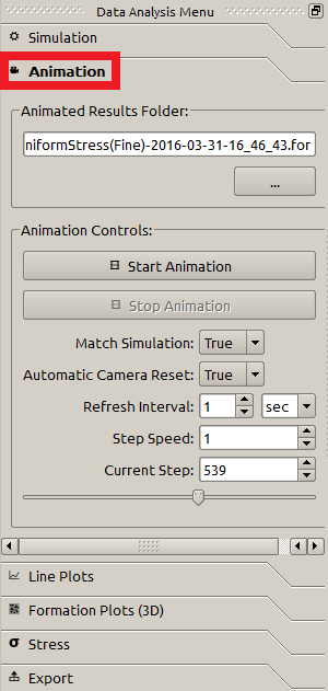
Figure 2: Animation tool box

By default, the Match Simulation checkbox is True. If it is True, then the most recent available data from the simulator will be plotted while the animation is running, ignoring the other parameters in this toolbox.

If the Match Simulation checkbox is False, or if the simulation is not running, then we can control the animation using the following parameters:

• Refresh Interval: How often, in real time, to update the plots.
• Step Speed: How fast it is in the animation between refreshes.
• Current Step: The time step the animation is currently at. This can be changed by editing the plot time text, or moving the slider directly below it.

Another controlling parameter is the Automatic Camera Rest that controls the size and angle from which the plot is presented. If it is True, the plot will be set to the default one at each refresh even the user changes it. On the other hand, if it is False, the plot will remain unchanged once the user changes it.

Plots¶

There are two plot toolboxes for the result plotting. One is the Line Plots , which also consists of two clusters of results to plot. One is the Global Properties (Fig 3) that plots an individual parameter (for example downhole pressure) during the whole simulation.

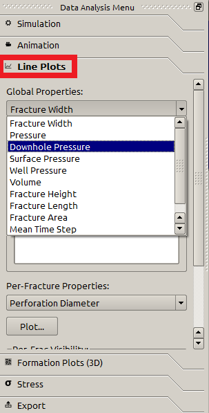
Figure 3: Line plot tool box - global properties

The Global Properties holds the Result Comparison list. Previous global results from the current project or other projects can be plotted against the current animation’s 2D data. To add a comparison, load (blue box in Fig 4) and select the project you want to compare, and check the box next to the data the user wants to compared. The compared data will be shown in the same colors as the current data, but with dotted lines.

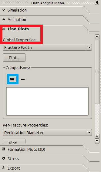
Figure 4: Line plot tool box - comparison

The other cluster is the Per-Frac Properties (Fig 5) that plots parameters at each injection sites (fractures).

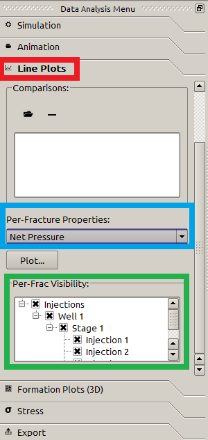
Figure 5: Line plot tool box - per-frac properties

If there are multiple fractures generated in the current running simulation, the user can hide or display the plotting of the parameters associated with certain fractures by checking the corresponding injections in the Per-Frac Visibility (green box in Fig 5) box.

Besides the Line Plots, The other plot toolbox is the Formation Plots toolboxes (Fig 6)

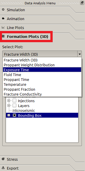
Figure 6: Line plot tool box

The Line plots show 2D result data, and Formation Plots show 3D result data. In both toolboxes, when a plot is selected with the drop down menu, click the Plot button to show that plot.

The Formation Plots menu contains the 3D Item Visibility tree. Using the checkboxes in this tree, different parts of the 3D plots can be shown or hidden. The fractures are numbered based on their creation time, and the layers are numbered with the top layer being Layer \(1\). Inside the items, the Bounds represents the smallest box that holds all the fractures (see Figure 7 for example)

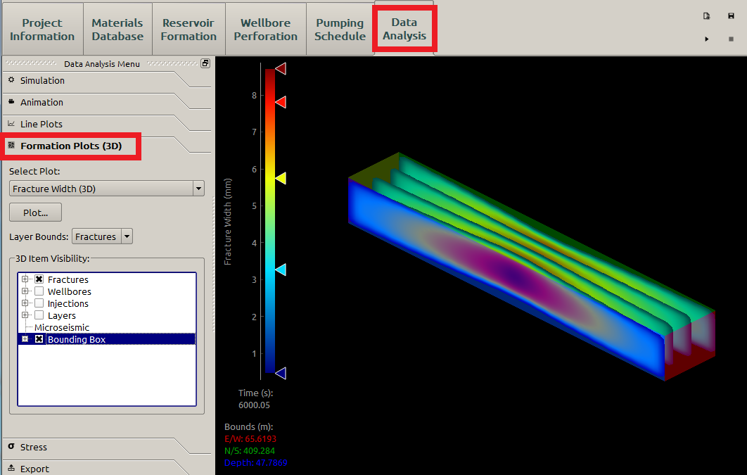
Figure 7: Bounding box

Stress¶

The Stress toolbox computes the resultant stress on defined planes during/after the simulation. Please notice that the stress inputs in Reservoir Formation panel and Reservoir Stress subpanel under the Wellbore Perforation are the initial stress conditions essentially, while the stress here is the output of the simulation.

Here presents an example of stress calculation of a project that generates four fractures (Figure 8). The FrackOptima simulator can only calculate stresses at the time when Calculate button of the Stress toolbox is clicked (Figure 9). It cannot be calculated dynamically with simulation running.

Before calculating the stress, it is recommended that users stop the animation, as shown in Figure 8, while the simulation is still running. Otherwise, it occupies huge CPU and memory resources.

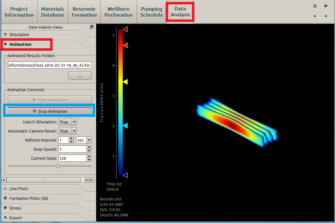
Figure 8: Stress calculation - Step 1

Then go to the Stress toolbox, insert a plane by clicking the “+” button, and define its orientation and position. After that we can choose which stress component is calculated and its properties in the Properties box, as displayed in Figure 9

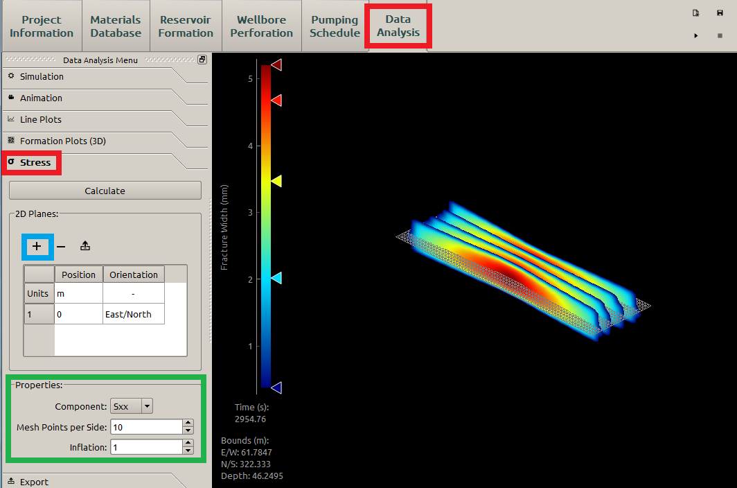
Figure 9: Stress calculation - Step 2

Inside the Properties box:

• Mesh Points per Side: number of the mesh points on the short side of the defined plane. Increasing this parameter yields refined mesh
• Inflation: this parameter defines the plane size. Denote Inflation as \(n\), then the plane size is \(n\) times of the corresponding dimensions of the Bounds. See Figure 10 for a refined mesh and enlarged plane.

The Properties must be defined before stress calculation. During the stress calculation the Properties cannot be changed.

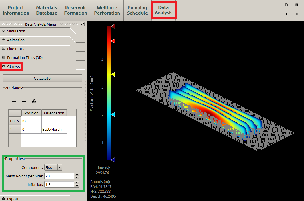
Figure 10: Stress Properties

After that, we can calculated the chosen stress by clicking Calculate button and the result is shown in Figure 11, in which the user changes the background from Dark to Light by right clicking the mouse and choosing the corresponding background in the subsequent context.

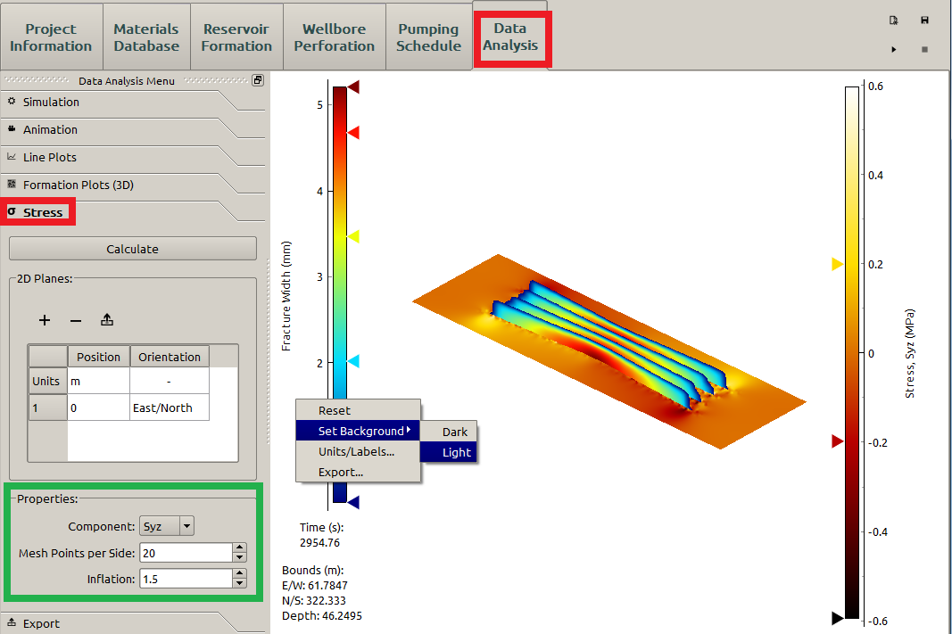
Figure 11: Stress calculation - Step 3 complete

To get a clearer view, the user can go to the Formation Plots(3D) toolbox and uncheck all the items in 3D Item Visibility (Figure 12).

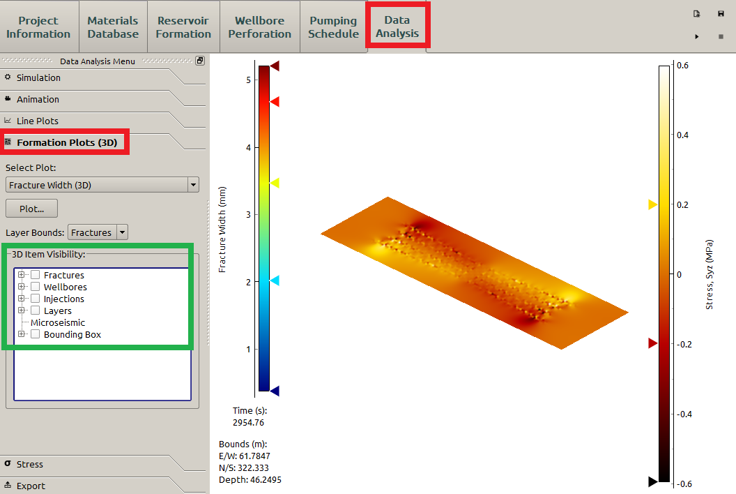
Figure 12: A clearer view of the stress distribution on a defined plane

Exporting¶

See the Exporting Result Data section.