Vector and Tensor Algebra¶

Vector¶

Introduction¶

A vector $\vec a$ (the red solid arrow in Figure 1) in a three dimensional space is denoted by:

(1)\[\begin{split}\vec a &= a_1 {\vec e}_1 + a_2 {\vec e}_2 + a_3 {\vec e}_3 \\ &= \sum_{i=1}^{3}a_i {\vec e}_i \\ &= a_i {\vec e}_i\end{split}\]

where,

$a_1$, $a_2$, $a_3$ or $a_i$ ($i=1,2,3$) are the three components of the vector $\vec a$. They represent the length of the projection of $\vec a$ with relation to the vector basis $[ {\vec e}_1, {\vec e}_2, {\vec e}_3 ]$ .

${\vec e}_i$ (the three short dashed arrow in Figure 1) is the vector basis of the vector $\vec a$ in a Cartesian rectangular coordinate system. The vector basis consists of all the independent vectors of a coordinate system, i.e. each other vector can be expressed as a weighted sum of these base vectors (Eqn. (1)). When the base vectors are mutually perpendicular, the basis is called orthogonal. If the orthogonal basis consists of mutually perpendicular unit vectors, it is called orthonormal. Here, we assume the basis $[{\vec e}_1, {\vec e}_2, {\vec e}_3]$ is orthonormal in the Cartesian rectangular coordinate.

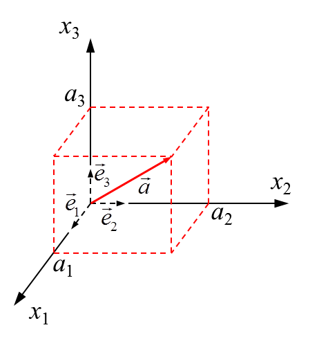
Figure 1: A vector in the Cartesian rectangular coordinate

The Einstein notation is then introduced to further simplify Eqn. (1).It is a notational convention that implies summation over a set of indexed terms in a formula, leading to a notational brevity. According to this convention , when an index variable appears twice in a single term and is not otherwise defined, it implies summation of that term over all the values of the index. Thus, Eqn. (1) can be simplified to:

(2)\[\begin{split}\vec a &= \sum_{i=1}^{3}a_i {\vec e}_i \\ &= a_i {\vec e}_i\end{split}\]

In Cartesian rectangular coordinate system (Figure 1), the base vectors ${\vec e}_i$ are constants. In other coordinate, for example polar coordinate systems, the base vectors may not be constant.

Basic Operations (Addition and Subtraction)¶

Following Eqn. (1), we can define two vectors in Eqn. (3) :

(3)\[\begin{split}\vec a &= a_1 {\vec e}_1 + a_2 {\vec e}_2 + a_3 {\vec e}_3 \\ \vec b &= b_1 {\vec e}_1 + b_2 {\vec e}_2 + b_3 {\vec e}_3 \\\end{split}\]

Then, a third vector $\vec c$ can be obtained by the addition or subtraction of $\vec a$ and $\vec b$:

(4)\[\begin{split}\vec c &= \vec a \pm \vec b \\ &= a_i {\vec e}_i \pm b_i {\vec e}_i \\ &= (a_i \pm b_i){\vec e}_i \\\end{split}\]

or more concisely:

(5)\[c_i = a_i \pm b_i\]

The Eqn. (5) is also called index notation.

Vector Operators (Dot/Cross product, Gradient, Divergence, Curl)¶

1. Dot product:

The dot product is defined in Eqn. (6)

(6)\[\begin{split}\vec a \cdot \vec b &= a_1 b_1 + a_2 b_2 + a_3 b_3 \\ &= \sum_{i=1}^{3}a_i b_i \\ &= a_i b_i \\\end{split}\]

The third row of Eqn. (6) is expressed by following the Einstein notation.

Because the dot product finally yields a scalar, it is sometimes called scalar product.

2. Cross product:

The cross product is defined in Eqn. (7):

(7)\[\vec a \times \vec b = \epsilon_{ijk} a_j b_k\]

where, the Levi-Civita symbol (also called Permutation symbol, or Alternating symbol) $\epsilon_{ijk}$ is defined as:

(8)\[\begin{split}\epsilon_{ijk} &= \frac{1}{2}(i-j)(j-k)(k-i) \\ &= \left\{ \begin{array}{ll} +1 & \textrm{if ($ijk$) is (123), (231) and (312)} \\ -1 & \textrm{if ($ijk$) is (321), (213) and (132)} \\ 0 & \textrm{Otherwise} \end{array} \right.\end{split}\]

Because $\epsilon_{ijk}$ is otherwise defined in Eqn. (8), thus Eqn. (7) does not follow Einstein notation. Substitution of Eqn. (8) into (7) yields a more explicit expression:

(9)\[\begin{split}\vec a \times \vec b &= (a_2b_3-a_3b_2){\vec e}_1 + (a_3b_1-a_1b_3){\vec e}_2 + (a_1b_2-a_2b_1){\vec e}_3 \\ &= \left| \begin{array}{ccc} {\vec e}_1 & {\vec e}_2 & {\vec e}_3 \\ a_1 & a_2 & a_3 \\ b_1 & b_2 & b_3 \\ \end{array} \right|\end{split}\]

The second row of Eqn. (9) is also called the determinant of a $3\times3$ matrix consisting of the $9$ same components. In other words, when we have a $3\times3$ matrix $\underset{\sim}{\textrm{A}}$ defined in (10):

(10)\[\begin{split}\underset{\sim}{\textrm{A}} = \left[ \begin{array}{ccc} a_1 & a_2 & a_3 \\ b_1 & b_2 & b_3 \\ c_1 & c_2 & c_3 \\ \end{array} \right ]\end{split}\]

The determinant of the matrix $\underset{\sim}{\textrm{A}}$ is:

(11)\[\begin{split}| \underset{\sim}{\textrm{A}} | &= \left| \begin{array}{ccc} a_1 & a_2 & a_3 \\ b_1 & b_2 & b_3 \\ c_1 & c_2 & c_3 \\ \end{array} \right| \\ &= a_1b_2c_3 + a_2b_3c_1 + a_3b_1c_2 - a_3b_2c_1 - a_2b_1c_3 - a_1b_3c_2\end{split}\]

Because the cross product finally yields a vector, it is sometimes called vector product.

3. Gradient:

In physics, it is necessary to determine changes of variables (scalars, vectors or tensors) with respect to the spatial position. An important operator used to determine these spatial derivatives is the gradient operator.

The gradient of a scalar function $f(x_1, x_2, x_3)$ is denoted by $\vec{\nabla} f$, where the nabla symbol $\vec{\nabla}$ denotes the vector differential operator. It points in the direction of the greatest rate change of the function $f$, and its magnitude is the slope of the graph in that direction. The notation $\textrm{grad}(f)$ is also commonly used for the gradient.

In a three-dimensional rectangular coordinate system, the expression of the gradient of $f(x_1, x_2, x_3)$ is obtained by fully differentiating $f$:

(12)\[\begin{split}\textrm{d}f &= \textrm{d}x_1\frac{\partial f}{\partial x_1} + \textrm{d}x_2\frac{\partial f}{\partial x_2} + \textrm{d}x_3\frac{\partial f}{\partial x_3} \\ &= (\textrm{d}\vec{x} \cdot \vec{e}_1)\frac{\partial f}{\partial x_1} + (\textrm{d}\vec{x} \cdot \vec{e}_2)\frac{\partial f}{\partial x_2} + (\textrm{d}\vec{x} \cdot \vec{e}_3)\frac{\partial f}{\partial x_3} \\ &= \textrm{d}\vec{x} \cdot \Bigg[ \vec{e}_1 \frac{\partial f}{\partial x_1} + \vec{e}_2 \frac{\partial f}{\partial x_2} + \vec{e}_3 \frac{\partial f}{\partial x_3} \Bigg] \\ &= \textrm{d}\vec{x} \cdot \big( \vec {\nabla}f \big)\end{split}\]

where,

(13)\[\begin{split}\vec x = \left[ \begin{array}{ccc} x_1 \\ x_2 \\ x_3 \\ \end{array} \right]\end{split}\]

The long expression inside the brackets in the third row of Eqn. (12) is the gradient of $f$:

(14)\[\begin{split}\vec {\nabla}f &= {\vec e}_1\frac{\partial f}{\partial x_1} + {\vec e}_2\frac{\partial f}{\partial x_2} + {\vec e}_3\frac{\partial f}{\partial x_3} \\ &= \sum_{i=1}^{3}{\vec e}_i\frac{\partial f}{\partial x_i} \\ &= {\vec e}_i\frac{\partial f}{\partial x_i} \\ &= {\underset{\sim}{\vec {\textrm{e}}}}^{\textrm{T}} \mathbf{\nabla} \\ &= \mathbf{\nabla}^\textrm{T} \underset{\sim}{\vec {\textrm{e}}}\end{split}\]

where, $\underset{\sim}{\vec {\textrm{e}}}$ and $\mathbf{\nabla}$ are both one dimensional matrices (vectors), and the superscript $\textrm{T}$ represents transposition, both of which will be introduced later.

(15)\[ \begin{align}\begin{aligned}\begin{split}\underset{\sim}{\vec {\textrm{e}}} = \left[ \begin{array}{ccc} {\vec e}_1 \\ {\vec e}_2 \\ {\vec e}_3 \\ \end{array} \right] \\\end{split}\\\begin{split}\mathbf{\nabla} = \left[ \begin{array}{ccc} \frac{\partial}{\partial x_1} \\ \frac{\partial}{\partial x_2} \\ \frac{\partial}{\partial x_3} \\ \end{array} \right] \\\end{split}\end{aligned}\end{align} \]

The third row of Eqn. (14) is expressed by following the Einstein notation.

For example, the gradient of the scalar function $f$ defined in (16):

(16)\[f = 3x_1 + 5x_2^4 - \textrm{sin}(x_3)\]

is:

(17)\[\begin{split}\vec{\nabla}f &= \frac{\partial f}{\partial x_1}{\vec e}_1 + \frac{\partial f}{\partial x_2}{\vec e}_2 + \frac{\partial f}{\partial x_3}{\vec e}_3 \\ &= 3{\vec e}_1 + 20x_2^3{\vec e}_2 - \textrm{cos}(x_3){\vec e}_3\end{split}\]

Note

The gradient operator $\vec{\nabla}$ is not a vector, because it has no length or direction. The gradient of a scalar function $f$ is a vector function $\vec{\nabla} f$.

For a vector function $\vec f$ defined in the form as in Eqn. (18)

(18)\[\vec f(x_1, x_2, x_3) = f_1(x_1, x_2, x_3) {\vec e}_1 + f_2(x_1, x_2, x_3) {\vec e}_2 + f_3(x_1, x_2, x_3) {\vec e}_3\]

where $f_1$, $f_2$, and $f_3$ are the scalar functions of $x_1$, $x_2$, and $x_3$.

The gradient of $\vec f$ is:

(19)\[\begin{split}\vec{\nabla} \vec f &= \Bigg( {\vec e}_1\frac{\partial}{\partial x_1} + {\vec e}_2\frac{\partial}{\partial x_2} + {\vec e}_3\frac{\partial}{\partial x_3} \Bigg) \big( f_1 {\vec e}_1 + f_2 {\vec e}_2+ f_3 {\vec e}_3 \big) \\ &= {\vec e}_1f_{1,1}{\vec e}_1 + {\vec e}_1f_{2,1}{\vec e}_2 + {\vec e}_1f_{3,1}{\vec e}_3 + \\ & \: \: \: \: \: \ {\vec e}_2f_{1,2}{\vec e}_1 + {\vec e}_2f_{2,2}{\vec e}_2 + {\vec e}_2f_{3,2}{\vec e}_3 + \\ & \: \: \: \: \: \ {\vec e}_3f_{1,3}{\vec e}_1 + {\vec e}_3f_{2,3}{\vec e}_2 + {\vec e}_3f_{3,3}{\vec e}_3 \\ &= \left[ \begin{array}{ccc} {\vec e}_1 & {\vec e}_2 & {\vec e}_2 \\ \end{array} \right] \left[ \begin{array}{ccc} \frac{\partial}{\partial x_1} \\ \frac{\partial}{\partial x_2} \\ \frac{\partial}{\partial x_3} \\ \end{array} \right] \left[ \begin{array}{ccc} f_1 & f_2 & f_2 \\ \end{array} \right] \left[ \begin{array}{ccc} {\vec e}_1 \\ {\vec e}_2 \\ {\vec e}_3 \\ \end{array} \right] \\ &= {\underset{\sim}{\vec {\textrm{e}}}}^{\textrm{T}} \big( \mathbf{\nabla} {\underset{\sim}{\textrm{f}}}^\textrm{T} \big) \underset{\sim}{\vec {\textrm{e}}} \\ &= {\vec e}_i{}f_{j,i}{\vec e}_j\end{split}\]

where,

(20)\[ \begin{align}\begin{aligned}\begin{split}{\underset{\sim}{\textrm{f}}} = \left[ \begin{array}{ccc} f_1 \\ f_2 \\ f_3 \\ \end{array} \right]\end{split}\\{}f_{i,j} = \frac{\partial f_i}{\partial x_j}\end{aligned}\end{align} \]

and $1\le i,j \le 3$.

The last row of Eqn. (19) is expressed by following the Einstein notation; and the second last row is expressed by following the matrix multiplication, which will be introduced later.

4. Divergence:

Divergence is a vector operator that produces a signed scalar field giving the quantity of a vector field’s source at each point. It represents the volume density of the outward flux of a vector filed from an infinitesimal volume around a given point. For example in the electrostatic filed due to a point charge (Figure 2):

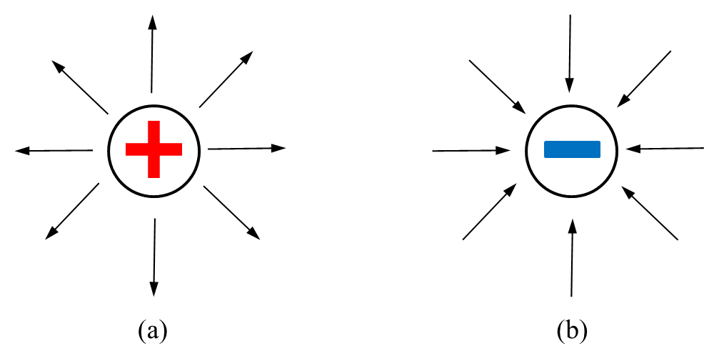
Figure 2: Electrostatic field divergence of a point charge: (a) positive charge, (b) negative charge

if the charge is positive, the electric field radiates outward, thus the divergence at the positive charge location is positive. The stronger the charge is, the larger the divergence is (for example, $1$ to $2$);

On a contrary, if the charge is negative, the electric field points inward , thus the divergence at the negative charge location is negative. The stronger the charge is, the smaller the divergence is (for example, $-1$ to $-2$)

In a three-dimensional rectangular coordinate system, a continuously differentiable vector function $\vec f$ can be expressed as in Eqn. (18), the divergence of $\vec f$ is denoted by $\textrm{div}\vec f$, and defined by:

(21)\[\begin{split}\textrm{div}\vec f &= \vec {\nabla} \cdot \vec f \\ &= \frac{\partial f_1}{\partial x_1} + \frac{\partial f_2}{\partial x_2} + \frac{\partial f_3}{\partial x_3} \\ &= \phantom{}f_{i,i}\end{split}\]

where, $\vec {\nabla}$ is the nabla symbol, and $\cdot$ is the dot product symbol. The last row of Eqn. (21) is expressed by following the Einstein notation.

Note

The divergence is the dot product of the vector operator $\vec{\nabla}$ and a vector function. It is a scalar function.

5. Curl:

The curl is a vector operator that characterizes the infinitesimal rotation of a point in a three dimensional vector field. Its direction is the axis of rotation, as determined by the right-hand rule, while its magnitude is the magnitude of the rotation. For example, if the velocity field forms a number of concentric circles whose center remains the same (Figure 3), the curl of the center points perpendicularly inwards to the plane of the rotation.

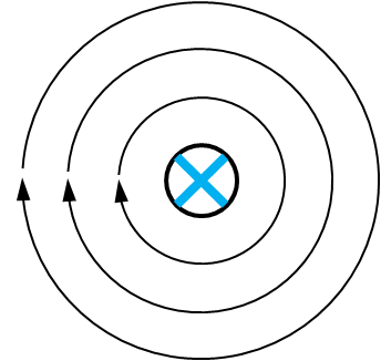
Figure 3: The concentric-circled velocity field and the inwards curl at the center

In a three-dimensional rectangular coordinate system, the curl of a continuously differentiable vector function $\vec f$ (Eqn. (18)) is denoted by $\textrm{curl}\vec f$, and defined by:

(22)\[\begin{split}\textrm{curl}\vec f &= \vec{\nabla} \times \vec f \\ &= \bigg(\frac{\partial f_3}{\partial x_2}- \frac{\partial f_2}{\partial x_3}\bigg){\vec e}_1 + \bigg(\frac{\partial f_1}{\partial x_3}- \frac{\partial f_3}{\partial x_1}\bigg){\vec e}_2 + \bigg(\frac{\partial f_2}{\partial x_1}- \frac{\partial f_1}{\partial x_2}\bigg){\vec e}_3 \\ &= \left| \begin{array}{ccc} {\vec e}_1 & {\vec e}_2 & {\vec e}_3 \\ \frac{\partial}{\partial x_1} & \frac{\partial}{\partial x_2} & \frac{\partial}{\partial x_3} \\ f_1 & f_2 & f_3 \\ \end{array} \right|\end{split}\]

where, $\vec{\nabla}$ is the nabla symbol, and $\times$ is the cross product symbol.

Note

The curl is the cross result of the vector operator $\vec{\nabla}$ and a vector function. It is a vector function.

6. Tensor Product (Dyad):

The tensor product of two vectors represents a dyad, which is a linear vector transformation ($\vec a \vec b$ in Figure 4). A dyad is a special tensor (to be discussed later), which explains the name of this product. Because it is often denoted without a symbol between the two vectors, it is also called open product.

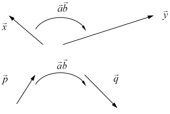
Figure 4: A dyad is a linear vector transformation

(23)\[\begin{split} \left\{ \begin{array}{ll} \vec a \vec b \cdot \vec x = \vec a \big( \vec b \cdot \vec x \big) = \vec y \\ \vec a \vec b \cdot \big( \alpha \vec x + \beta \vec p \big) = \alpha \vec a \vec b \cdot \vec x + \beta \vec a \vec b \cdot \vec p = \alpha \vec y + \beta \vec q \end{array} \right.\end{split}\]

The tensor product is not commutative. Swapping the vectors leads to the conjugate or transpose dyad. If the dyad is commutative, it is called symmetric:

(24)\[\begin{split} \left\{ \begin{array}{ll} \textrm{conjugated dyad}: & \big( \vec a \vec b \big)^c = \vec b \vec a \neq \vec a \vec b\\ \textrm{symmetric dyad}: & \big( \vec a \vec b \big)^c = \vec a \vec b \end{array} \right.\end{split}\]

Matrix¶

Introduction¶

A $\textrm{m}\times\textrm{n}$ matrix $\underset{\sim}{\textrm{K}}$ is a collection of entries with $\textrm{m}$ rows and $\textrm{n}$ columns:

(25)\[\begin{split}\underset{\sim}{\textrm{K}} = \left[ \begin{array}{ccc} \textrm{k}_{11} & \textrm{k}_{12} & \ldots & \textrm{k}_{1\textrm{n}} \\ \textrm{k}_{21} & \textrm{k}_{22} & \ldots & \textrm{k}_{2\textrm{n}} \\ \vdots & \vdots & \ddots & \vdots \\ \textrm{k}_{\textrm{m}1} & \textrm{k}_{\textrm{m}2} & \ldots & \textrm{k}_\textrm{mn} \\ \end{array} \right]\end{split}\]

When $\textrm{m}=\textrm{n}$, $\underset{\sim}{\textrm{K}}$ is called square matrix.

A vector can be viewed as a one column or one matrix:

(26)\[\begin{split}\vec a = \underset{\sim}{\textrm{a}} = \left[ \begin{array}{ccc} a_1 \\ a_2 \\ \vdots \\ a_\textrm{m} \\ \end{array} \right]\end{split}\]

or

(27)\[\begin{split}\vec a = \underset{\sim}{\textrm{a}} = \left[ \begin{array}{ccc} a_1 & a_2 & \ldots & a_\textrm{n} \\ \end{array} \right]\end{split}\]

The transpose of a matrix $\underset{\sim}{\textrm{K}}$ is another matrix ${\underset{\sim}{\textrm{K}}}^\textrm{T}$ created by reflecting $\underset{\sim}{\textrm{K}}$ over its main diagonal:

(28)\[ \begin{align}\begin{aligned}\begin{split}\underset{\sim}{\textrm{K}} = \left[ \begin{array}{ccc} \textrm{k}_{11} & \textrm{k}_{12} & \ldots & \textrm{k}_{1\textrm{n}} \\ \textrm{k}_{21} & \textrm{k}_{22} & \ldots & \textrm{k}_{2\textrm{n}} \\ \vdots & \vdots & \ddots & \vdots \\ \textrm{k}_{\textrm{m}1} & \textrm{k}_{\textrm{m}2} & \ldots & \textrm{k}_\textrm{mn} \\ \end{array} \right] \\\end{split}\\\Downarrow\\\begin{split}{\underset{\sim}{\textrm{K}}}^\textrm{T} = \left[ \begin{array}{ccc} \textrm{k}_{11} & \textrm{k}_{21} & \ldots & \textrm{k}_{\textrm{m}1} \\ \textrm{k}_{12} & \textrm{k}_{22} & \ldots & \textrm{k}_{\textrm{m}2} \\ \vdots & \vdots & \ddots & \vdots \\ \textrm{k}_{1\textrm{n}} & \textrm{k}_{2\textrm{n}} & \ldots & \textrm{k}_\textrm{mn} \\ \end{array} \right]\end{split}\end{aligned}\end{align} \]

and particularly:

(29)\[\begin{split}\left[ \begin{array}{ccc} a_1 & a_2 & \ldots & a_\textrm{n} \\ \end{array} \right]^\textrm{T} = \left[ \begin{array}{ccc} a_1 \\ a_2 \\ \vdots \\ a_\textrm{n} \\ \end{array} \right]\end{split}\]

Thus, the transpose of a $\textrm{m}\times\textrm{n}$ matrix $\underset{\sim}{\textrm{K}}$ is a $\textrm{n}\times\textrm{m}$ matrix ${\underset{\sim}{\textrm{K}}}^\textrm{T}$ . The $i$ th row, $j$ th column entry of ${\underset{\sim}{\textrm{K}}}^\textrm{T}$ is the $j$ th row, $i$ th column entry of $\underset{\sim}{\textrm{K}}$ :

(30)\[\left[ \begin{array}{ccc} {\underset{\sim}{\textrm{K}}}^\textrm{T} \end{array} \right]_{ij} = \left[ \begin{array}{ccc} \underset{\sim}{\textrm{K}} \end{array} \right]_{ji}\]

There is a special matrix denoted by $\underset{\sim}{\textrm{I}}$ and called Identity Matrix which is often involved in tensor algebra. It is a square matrix with ones on the main diagonal and zeros elsewhere:

(31)\[\begin{split}\underset{\sim}{\textrm{I}} = \left[ \begin{array}{ccc} 1 & 0 & \ldots & 0 \\ 0 & 1 & \ldots & 0 \\ \vdots & \vdots & \ddots & \vdots \\ 0 & 0 & \ldots & 1 \\ \end{array} \right]\end{split}\]

Basic Operations¶

1. Addition and Subtraction

The addition and subtraction can only be applied on the two matrices of the same size. If the matrices $\underset{\sim}{\textrm{A}}$ and $\underset{\sim}{\textrm{B}}$ are both of size $\textrm{m}\times\textrm{n}$, the addition/subtraction leads to a new matrix in which each element is calculated entrywise:

(32)\[ [\underset{\sim}{\textrm{A}} \pm \underset{\sim}{\textrm{B}}]_{ij} = [{}A_{ij} \pm {}B_{ij}]\]

where, ${}A_{ij}$ and ${}B_{ij}$ are entries of the matrices $\underset{\sim}{\textrm{A}}$ and $\underset{\sim}{\textrm{B}}$, respectively.

If $\underset{\sim}{\textrm{A}}$ and $\underset{\sim}{\textrm{B}}$ are of different sizes, they cannot be added or subtracted.

2. Scalar Multiplication

Scalar multiplication yields the product of a scalar number $c$ and a matrix $\underset{\sim}{\textrm{A}}$. It is calculated by multiplying every entry of $\underset{\sim}{\textrm{A}}$ by $c$:

(33)\[ [c\underset{\sim}{\textrm{A}}]_{ij} = c \cdot [\underset{\sim}{\textrm{A}}]_{ij}\]

3. Matrix Multiplication

Matrix multiplication of two matrices is defined if and only if the number of columns of the left matrix is the same as the number of rows of the right matrix. If $\underset{\sim}{\textrm{A}}$ is an $\textrm{m}\times\textrm{n}$ matrix and $\underset{\sim}{\textrm{B}}$ is an $\textrm{n}\times\textrm{p}$ matrix, then their matrix product $\underset{\sim}{\textrm{A}} \underset{\sim}{\textrm{B}}$ is the $\textrm{m}\times\textrm{p}$ matrix whose entries are given by dot product of the corresponding row of $\underset{\sim}{\textrm{A}}$ and the corresponding column of $\underset{\sim}{\textrm{B}}$:

(34)\[\begin{split} [\underset{\sim}{\textrm{A}} \underset{\sim}{\textrm{B}}]_{ij} &= {}A_{i1} {}B_{1j} +{}A_{i2} {}B_{2j} + ... {}A_{i\textrm{n}} {}B_{\textrm{n}j} \\ &= \sum_{r=1}^{\textrm{n}}{}A_{ir} {}B_{rj} \\ &= {}A_{ir} {}B_{rj}\end{split}\]

where, $1\le i \le \textrm{m}$, $1\le j \le \textrm{p}$, and $1\le r \le \textrm{n}$. The third row of Eqn. (34) is expressed by following the Einstein notation.

Tensor¶

Introduction and second-order tensor¶

A scalar function $f$ takes a scalar variable $x$ as input and yields another scalar variable $y$:

(35)\[y=f(x) \: \: \: \: \textrm{or} \: \: \: \: x \xrightarrow{f} y\]

Such a function is also called a projection.

Both input and output can also be vectors instead of scalars. A tensor is the equivalent of the function $f$ in this case. Compared to the arbitrary scalar function $f$, a tensor ($\mathbf{A}$ in Eqn. (36)) is special because it is always linear :

(36)\[\vec y = \mathbf{A} \cdot \vec x \: \: \: \: \textrm{or} \: \: \: \: \vec x \xrightarrow{\mathbf{A}} \vec y\]

The tensors introduced here and used mostly in engineering are second-order tensors, which can be written as the summation of a infinite number of dyads:

(37)\[\begin{split}\mathbf{A} &= \alpha_1 {\vec a}_1 {\vec b}_1 + \alpha_2 {\vec a}_2 {\vec b}_2 + \alpha_3 {\vec a}_3 {\vec b}_3 + .. \\ &= \sum_{i=1}^{\infty}\alpha_i {\vec a}_i {\vec b}_i \\ &= \alpha_i {\vec a}_i {\vec b}_i\end{split}\]

where the third row of Eqn. (37) is expressed by following the Einstein notation.

Components of a second-order tensor¶

Under the three-dimensional Cartesian rectangular coordinate with the orthonormal vector basis $[{\vec e}_1, {\vec e}_2, {\vec e}_3]$ (Figure 1), the components of the second-order $\mathbf{A}$ can be stored in a $3\times3$ matrix $\underset{\sim}{\textrm{A}}$:

(38)\[\begin{split}\mathbf{A} &= \alpha_1 {\vec a}_1 {\vec b}_1 + \alpha_2 {\vec a}_2 {\vec b}_2 + \alpha_3 {\vec a}_3 {\vec b}_3 + ... \\ &= \alpha_1( {}a_{11}{\vec e}_1 +a_{12}{\vec e}_2 +a_{13}{\vec e}_3) ( {}b_{11}{\vec e}_1 +b_{12}{\vec e}_2 +b_{13}{\vec e}_3) + \\ & \: \: \: \: \: \ \alpha_2( {}a_{21}{\vec e}_1 +a_{22}{\vec e}_2 +a_{23}{\vec e}_3) ( {}b_{21}{\vec e}_1 +b_{22}{\vec e}_2 +b_{23}{\vec e}_3) + \\ &= {}A_{11}{\vec e}_1{\vec e}_1 +A_{12}{\vec e}_1{\vec e}_2 +A_{13}{\vec e}_1{\vec e}_3 + \\ & \: \: \: \: \: \ {}A_{21}{\vec e}_2{\vec e}_1 +A_{22}{\vec e}_2{\vec e}_2 +A_{23}{\vec e}_2{\vec e}_3 + \\ & \: \: \: \: \: \ {}A_{31}{\vec e}_3{\vec e}_1 +A_{32}{\vec e}_3{\vec e}_2 +A_{33}{\vec e}_3{\vec e}_3 \\ &= \left[ \begin{array}{ccc} {\vec e}_1 & {\vec e}_2 & {\vec e}_2 \\ \end{array} \right] \left[ \begin{array}{ccc} {}A_{11} & {}A_{12} & {}A_{13} \\ {}A_{21} & {}A_{22} & {}A_{23} \\ {}A_{31} & {}A_{32} & {}A_{33} \\ \end{array} \right] \left[ \begin{array}{ccc} {\vec e}_1 \\ {\vec e}_2 \\ {\vec e}_3 \\ \end{array} \right] \\ &= {\underset{\sim}{\vec {\textrm{e}}}}^{\textrm{T}} \underset{\sim}{\textrm{A}} \underset{\sim}{\vec {\textrm{e}}}\end{split}\]

where,

(39)\[\begin{split}{}A_{ij} &= \alpha_1 {}a_{1i} {}b_{1j} + \alpha_2 {}a_{2i} {}b_{2j} + ... \\ &= \sum_{r=1}^{\infty}\alpha_r {}a_{ri} {}b_{rj} \\ &= \alpha_r {}a_{ri} {}b_{rj}\end{split}\]

where the third row of Eqn. (39) is expressed by following the Einstein notation.