KGD Hydraulic Fracturing Model¶

Introduction¶

The Kristianovich-Geertsma-de Klerk (KGD) radial model is a classic 2D hydraulic fracturing model, named in honor of three researchers who contributed to it. [1] The following assumptions are used in the model: [2]

The formation is an infinite, homogeneous, isotropic, linear elastic medium characterized by Young’s modulus \(E\), Poisson’s ratio \(\nu\) and toughness \(K_{Ic}\).

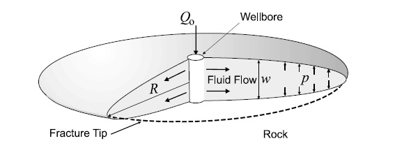
Figure 1: Schematic view of the KGD radial model geometries

The fracture is assumed to be radially symmetric and generated from a point-source at its center. The periphery of the fracture is circular (penny-shaped), as shown in Figure 1. [3]
The fracturing fluid is Newtonian with viscosity \(\mu\). It is injected with a constant volumetric flow rate \(Q_0\), and its flow is laminar. Gravitational effects are not taken into account.

The circular fracture propagation is expected from injections through a narrow band of perforations which form a point source. Because we are neglecting gravitational effects, the fracture propagation plane can be at any angle with respect to the wellbore [2]. A set of possible injection and wellbore parameters for FrackOptima can be specified in the Injections and Wells subpanels of the Wellbore Perforation panel, as shown in Figure 2 and Figure 3.

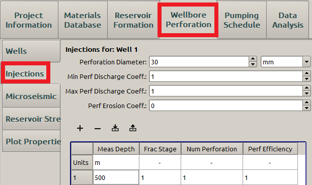
Figure 2: Input the injection location parameters

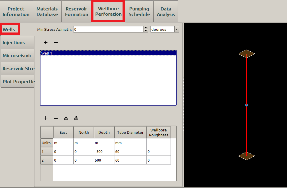
Figure 3: Input the wellbore location parameters

Neither the wellbore friction nor the perforation erosion is considered here, so the Wellbore Roughness and Perforation Erosion Coefficient are both \(0\).

Geertsma-de Klerk equation¶

The governing equations for the KGD model without fluid leakoff are two integral equations. One is the Poisseuille equation relating the fluid-pressure gradient to the fracture width:

(1)\[p_0 - p = \frac{6\mu Q_0}{\pi}\int_{f_\mathrm{Rw}}^{f_R} \frac{df_R}{f_R w^3}\]

where:

\(R\) is the maximum extent of the fracture
\(f_R = r/R\) represents the fraction of the fracture extent \(r\)
\(f_{Rw} = R_w/R\) represents the fraction of the wellbore radius \(R_w\)
\(p_0\) is the downhole pressure.
\(w\) is the local fracture width

The other equation is the Sneddon’s elasticity equation, which relates the fracture width \(w\) and fracture radius \(R\):

(2)\[w = \frac{4(1-\nu)R}{\pi G} \left( \int_{f_\mathrm{Rw}}^1 \frac{df_2}{\sqrt{f_2^2 - f_R^2}} \int_{f_\mathrm{Rw}}^{f_2} \frac{f_1p(f_1)df_1}{\sqrt{f_2^2 - f_R^2}} - S\sqrt{1-f_R^2} \right)\]

where \(G\) is the shear modulus of the formation, \(S\) is the tectonic stress normal to the fracture plane, and \(f_1\) and \(f_2\) are dummy fractions of the fracture extension. To make the analytical approximations available for the two equations, the two researchers make some extra assumptions: [2]

The Barenblatt’s tip condition applies for the fracture. It states that that the tip closes smoothly and the pressure is zero near the tip. The fracture shape is approximately parabolic except near the tip.
A constant average \(\bar{w}\) is assumed, as shown in Figure 4, up to a critical radius \(R_0\), beyond which Barenblatts tip condition applies. Thus, the pressure distribution is logarithmic according to Eqn (1), except near the tip. \(R_0\) is given by:

\[ \begin{align}\begin{aligned}f_\mathrm{R_0} = 1-\frac{2}{15}\frac{G}{R} \left( \frac{\mu Q_0}{S^4} \right)^{1/3}\\w = \bar{w}\end{aligned}\end{align} \]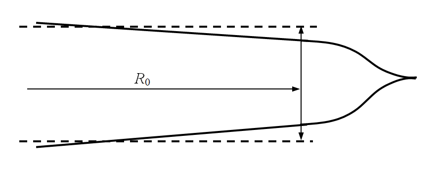

Figure 4: The Barenblatt’s tip condition and a constant average \(\bar{w}\) for approximation
Assuming zero pressure at the tip makes it impossible to define the stress intensity factor, so that the formation toughness cannot be taken into account. [4] Geertsma and de-Klerk argue that the formation toughness is negligible for large fractures in the practical range, and the tip processes dominate the fracture propagation [2] [3].

Based on the extra assumptions, and assuming Poisson’s ratio \(\nu = 0.25\), the fracture width at the wellbore \(w_0\) is approximated as:

(3)\[w_0=2.56\left( \frac{\mu Q_0R}{E'} \right)^{\frac{1}{4}}\]

Eq. (3) can also be obtained by replacing G in Equation 12 of Ref [2] with the plane strain Young’s modulus \(E' =\frac{E}{1-\nu^2}\).

The wellbore net pressure equation without leakoff is approximated as:

(4)\[p_0=S-\frac{5}{4\pi}\frac{G w_0}{R}\ln \frac{R_w}{R}\]

When fluid leakoff is taken into account, Carter’s equation is adopted to model the leakoff process:

\[Q_L=C_L\int_0^t\frac{dA}{dt_0}\frac{dt_0}{\sqrt{t-t_0}}\]

where \(Q_L\) is the fluid leakoff volumetric rate, \(C_L\) is the leakoff coefficient, \(A\) is the total exposed surface area, and \(t_0\) is the time at which the point is exposed.

Applying volume conservation yields:

\[Q_0=\frac{3}{5}\pi {w_0}\frac{dR^2}{dt}+2\pi {C_L} \int_0^t\frac{dR^2}{dt_0}\frac{dt_0}{\sqrt{t-t_0}}\]

With large leakoff, the analytical approximation can be derived by using the constant average width \(\bar{w}\):

(5)\[R = \frac{1}{\pi} \left( \frac{Q_0^2 t}{C_L^2} \right)^{1/4}\]

Note

The Geertsma-de Klerk equation (Eqns (3), (4), and (5)) are the approximations to the KGD model based on the Barenblatt’s tip condition and constant average width adoption.

Dimensionless analysis without leakoff¶

The Geertsma-de Klerk equations indicate that the formation toughness is negligible. [2] Some other researchers came to the opposite conclusion by asserting the ratio of the energy used to create new fracture surfaces to energy dissipated from viscous fluid flow helps decide if toughness can be neglected. If the ratio is small, toughness can be neglected, and if it is large, we must take toughness into account. [3] For the KGD radial model without leakoff, this criterion yields a critical value called a dimensionless toughness \(\kappa\), which is the only parameter contained in the scaled equations that determines the three different regimes for the dimensionless analysis of the KGD radial model: [3]

viscosity-dominated regime (\(\kappa = 0\)): the toughness may be neglected
toughness-dominated regime (\(\kappa = \infty\)): the viscosity may be neglected
transient regime: both parameters have to be taken into account

The dimensionless toughness \(\kappa\) is defined as:

\[\kappa = K'\left( \frac{t^2}{\mu'^5 Q_0^3 E'^{13}} \right)^\frac{1}{18}\]

where

\(K'= 4 \sqrt{\frac{2}{\pi}}K_{Ic}\)
\(\mu' = 12\mu\)
\(E' = \frac{E}{1-\nu^2}\)
\(t\) represents the injection time

The dimensionless analysis of the KGD radial model replaces Barenblatt’s tip condition with lubrication theory, so the inaccuracy due to the adoption of a constant average width in the integral governing equations can be avoided. In addition, the fracture tip becomes blunt and the net pressure at the tip is not zero, making the toughness involved in the solution. Hence, the fluid pressure governing equation (Eqn (1)) is replaced by the non-linear PDE from lubrication theory, while Sneddon’s Eqn (2) still holds:

(6)\[\frac{\partial w}{\partial t} = \frac{1}{\mu'} \frac{1}{r} \frac{\partial}{\partial r}\left( r w^3 \frac{\partial p}{\partial r} \right)\]

The derivation of the above PDE can be found here.

The following scaling forms are applied on the governing equations:

\[\begin{split}\left\{ \begin{align} & R(t)=L(t)\gamma (\lambda (t)) \\ & w(r,t)=\varepsilon (t)L(t)\Omega (\rho ,\lambda (t)) \\ & p(r,t)=\varepsilon (t)E'\Pi (\rho ,\lambda (t)) \\ \end{align} \right.\end{split}\]

where \(\rho=r/R\), \(\gamma\), \(\Omega\), and \(\Pi\) are dimensionless fracture radius, opening, pressure, respectively; \(\lambda (t)\) is a dimensionless parameter depending on \(t\) monotonically and \(L\) is the length scale.

Analysis of the scaled governing equations indicates that the solution is self-similar for the two limiting cases: the viscosity-dominated regime (\(\kappa = 0\)) and the toughness-dominated regime (\(\kappa = \infty\)). Hence it is independent of the initial conditions [3]. Then, asymptotic analytical solutions (\(\gamma\), \(\Omega\), and \(\Pi\)) can be approximated when \(\kappa\) is less than 1 or larger than 3.5 [3]. Among those analytical solutions, the dimensionless radius \(\gamma\) can be expressed in an explicit closed form:

\[\begin{split}\gamma \approx \left\{ \begin{align} & 0.6976, \kappa \le 1 \\ & \left( \frac{3}{\pi \sqrt{2}} \right)^{\frac{2}{5}} \kappa^{-\frac{2}{5}} - \frac{544}{75\pi^2} \kappa^{-4}, \kappa \ge 3.5 \\ \end{align} \right.\end{split}\]

The numerical dimensionless radius \(\gamma_f\) can be calculated by:

\[\gamma_f = \frac{R_f}{L_m}\]

where

\[L_m(t)=\left( \frac{Q_0^3 E't^4}{\mu'} \right)^\frac{1}{9}\]

The FrackOptima fracture radius \(R_f\) can be obtained after running the simulation.

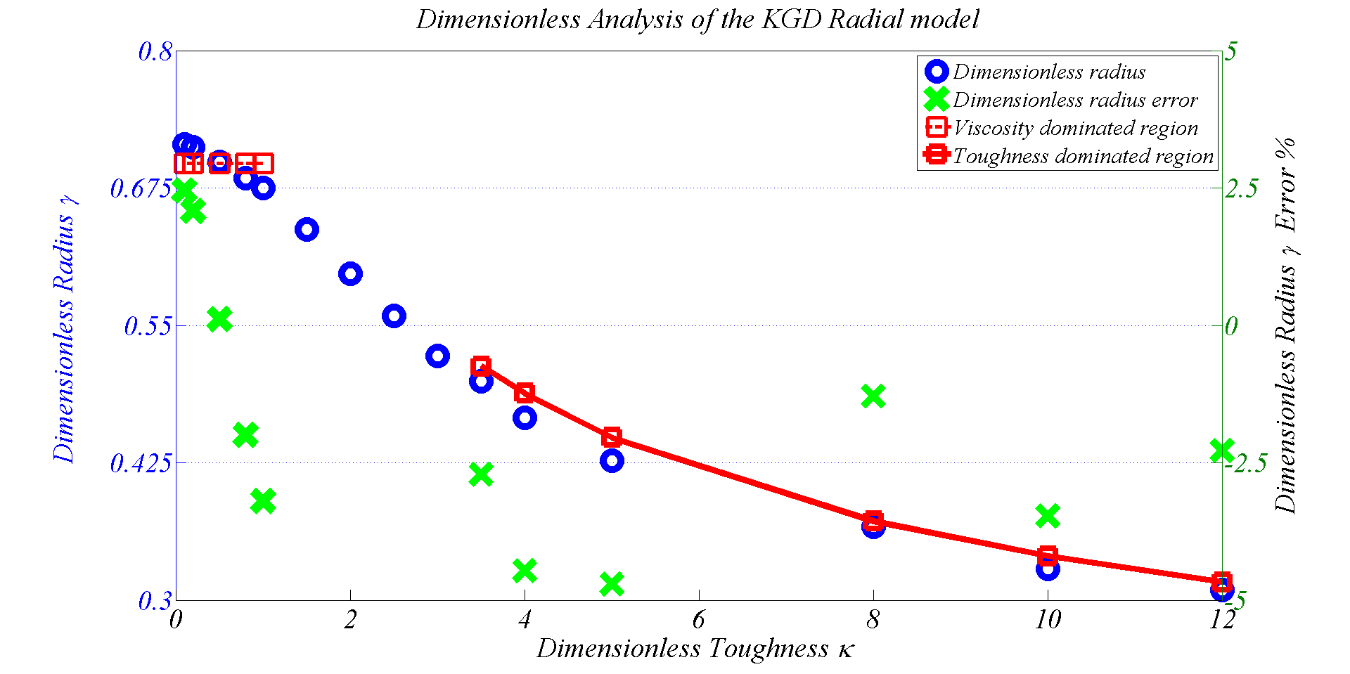
Figure 5: The comparison of the FrackOptima result and the analytical one.

The comparison between FrackOptima and the analytical solution is shown in Figure 5, which indicates a good match between those two results. The error is defined as:

\[Error = \frac{\gamma_f - \gamma}{\gamma} \times 100\%\]

Note

The dimensionless analysis of the KGD radial model without leakoff is an improved approximation because the first-order asymptotic analysis, which replaces the Barenblatt’s tip condition with the lubrication theory, accounts for toughness and the error due to the constant average width assumption is avoided.

Static analysis without leakoff¶

The exact solution to a static penny-shaped fracture without leakoff under constant net normal pressure \(p_0\) is given by the following equations:

The fracture radius:

\[R = \left( \frac{3E' Q_0 t}{8 \sqrt{\pi} K_\mathrm{Ic}} \right)^{0.4}\]
The wellbore net pressure:

\[p_0 = \frac{\sqrt{\pi} K_\mathrm{Ic}}{2 \sqrt{R}}\]
The wellbore fracture width:

\[w_0 = \frac{8 p_0 R}{\pi E'}\]

The static analysis can be carried out by setting long enough shut-in time after the injection so that the fracture will not grow. The two examples, one of which is for viscosity-dominated regime and the other one is for toughness-dominated regime are presented in Table 1 and Table 2, respectively.

FrackOptima result¶

The toughness-dominated region¶

Example 1

Young’s modulus \(E =8.51743(\textrm{GPa})\)
Poisson ratio \(\nu =0.25\)
Rock toughness \(K_{Ic} =8(\textrm{MPa} \bullet \sqrt{\textrm{m}})\)
Fluid viscosity \(\mu =0.001(\textrm{Pa}\bullet \textrm{sec})\),
Pumping rate \(Q_0 =0.26(\textrm{m}^3/\textrm{sec})\)
Injection time \(t_{injection} =125.5(\textrm{sec})\),
Total time: \(t_{end} =300(\textrm{sec})\) .

Thus, the dimensionless toughness \(\kappa = 12\) in the toughness-dominated regime.

Reservoir Formation¶

Firstly, we need to specify reservoir parameters in the “Reservoir Formation” panel. The formation interface depths are specified in the “Interface” subpanel as shown in Figure 6.

Two important parameters are the element size along the layer and across the layer, which determine the number of elements used in the simulation. Larger values for these parameters result in a coarse element mesh which may decrease the accuracy of the simulation. Conversely, a more refined mesh increases the time it takes to perform the simulation. Therefore, users need to determine an appropriate element size based on the specific case. Here \(\textrm{5 m}\) is chosen for both directions.

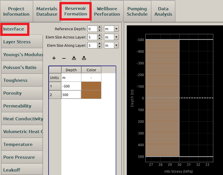
Figure 6: Input the interface parameters.

Next, we specify the stress and pore pressure profiles in the “Stress” and “Pore Pressure” subpanels, as shown in Figure 7 and Figure 8. We use the following constant profiles:

Min Stress: \(\textrm{30 MPa}\)
Max Stress: \(\textrm{33 MPa}\)
Pore Pressure: \(\textrm{20 MPa}\)

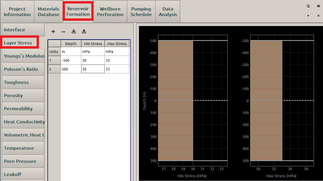
Figure 7: Input the formation stress.

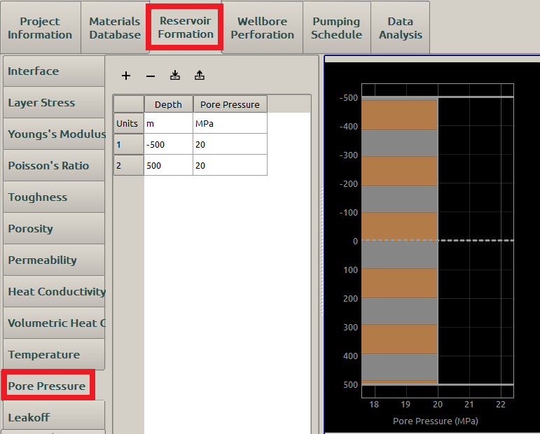
Figure 8: Input the formation pore pressure.

The formation temperature is specified in the Temperature subpanel as shown in Figure 9. Since False is set for the Has crosslinker option of the fluid as in Figure 12, there is no temperature effect on fluid viscosity. Here a uniform temperature profile is input.

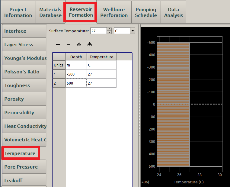
Figure 9: Input the formation temperature parameters

In addition, the KGD radial model assumes a homogeneous, isotropic formation, so the other formation properties are evaluated by Table 1.

Table 1: Formation properties of the KGD model¶
	Depth	Young’s Modulus	Poisson Ratio	Toughness	Porosity	Permeability	Heat Conductivity	Volumetric Heat Capacity	Leakoff	Spurtloss
Units	\(\textrm{m}\)	\(\textrm{MPa}\)		\(\mathrm{MPa} \bullet \sqrt{\mathrm{m}}\)		\(\textrm{m}^2\)	\(\textrm{W/(m}\bullet\textrm{K)}\)	\(\textrm{J/(m}^3 \bullet\textrm{K)}\)	\(\textrm{m/s}^{0.5}\)	\(\textrm{m}\)
	\(\textrm{-500}\)	\(\textrm{8.51743}\)	\(\textrm{0.25}\)	\(\textrm{8}\)	\(\textrm{0.05}\)	\(\textrm{0.01}\)	\(\textrm{1.5}\)	\(\textrm{2e6}\)	\(\textrm{0}\)	\(\textrm{0}\)
	\(\textrm{500}\)	\(\textrm{8.51743}\)	\(\textrm{0.25}\)	\(\textrm{8}\)	\(\textrm{0.05}\)	\(\textrm{0.01}\)	\(\textrm{1.5}\)	\(\textrm{2e6}\)	\(\textrm{0}\)	\(\textrm{0}\)

An example of the Young’s Modulus input is shown in Figure 10.

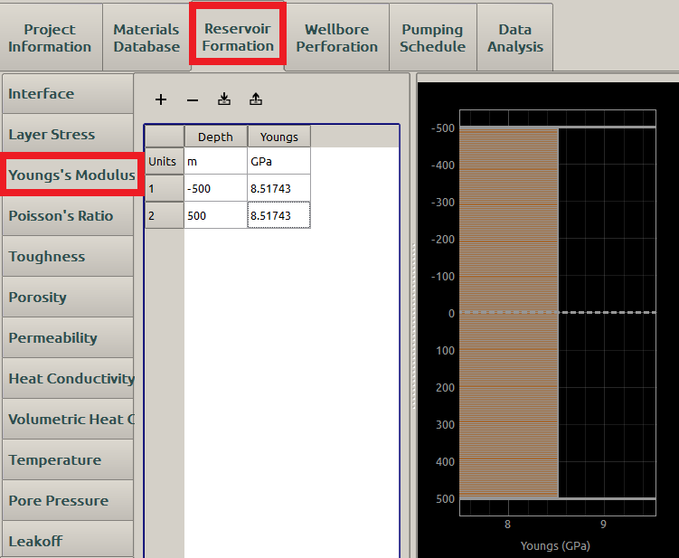
Figure 10: Input the rock Young’s modulus

Material Database¶

After specifying the formation properties, the fluid parameters are entered in the Fluids subpanel of the Material Database panel, as shown in Figure 11. Because the fluid is assumed to behave as a Newtonian laminar flow so that the Behavior Index value should be \(\textrm{1}\). In addition, the fluid involved in KGD model is assumed weightless, thus the Density is set as \(0\). And we set the Has Crosslinker as False , as displayed in Figure 12 so that the temperature effect on fluid viscosity is excluded.

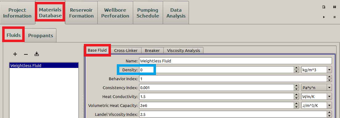
Figure 11: Input the fluid parameters.

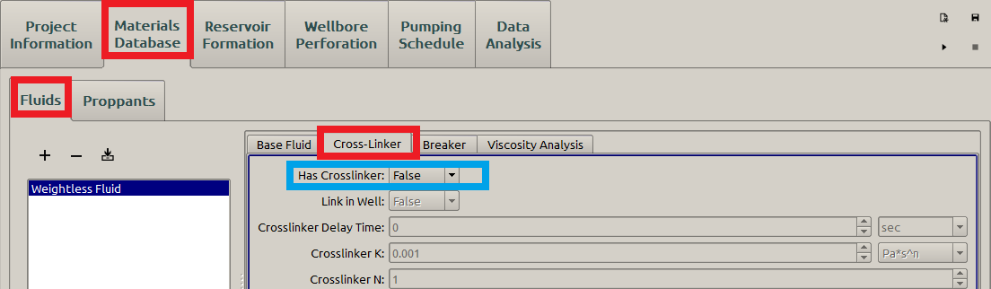
Figure 12: Form view of the fluid parameters.

The proppant parameters are specified as shown in Figure 13, although it is not involved in the KGD model. If the proppant is not specified here, the Pumping Schedule panel yields an error indicator.

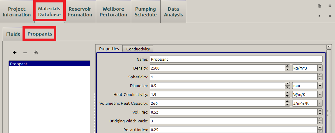
Figure 13: Input the proppant parameters

Pumping schedule¶

The Wellbore Perforation inputs have already been shown in the Figure 3 and Figure 2. After the wellbore perforation parameters, the inputs of the Pumping Schedule panel may be specified as shown in Figure 14. The proppant menu marked in the green box must be specified with the one defined as in Figure 13 otherwise an error indicator appears. The parameters associated with proppant are all set to zero because it is not involved within the KGD model.

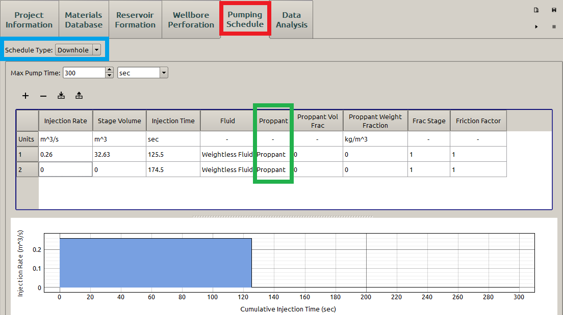
Figure 14: Input the pumping schedule parameters.

In addition, the Injection Time represents the duration of each pumping schedule defined here. In this example, the fluid is injected for \(125.5(sec)\) and then it is kept shut-in for \(174.5(sec)\) so that the total time is \(300(sec)\).

Since the KGD is a theoretical model, we can simply set the Schedule Type as Downhole without the interpretation.

Having input all the parameters, we can start the computation and get the result as shown in the Table 1:

Comparison of the FrackOptima results and the analytical one in toughness-dominated regime¶
Type	Radius (m)	Net Pressure (MPa)	Width (mm)
Analytical	\(36.12\)	\(1.1797\)	\(11.9427\)
FrackOptima	\(35\)	\(1.2560\)	\(12.3851\)
Error \(\%\)	\(-3.10\)	\(6.47\)	\(3.57\)

We also get results for the viscosity-dominated regime with the Example 2.

Example 2¶

Young’s modulus \(E =31.9233 (\textrm{GPa})\)
Poisson ratio \(\nu =0.25\)
Rock toughness \(K_{Ic} =1(\textrm{MPa} \bullet \sqrt{\textrm{m}})\)
Fluid viscosity \(\mu =0.5(\textrm{Pa}\bullet \textrm{sec})\),
Pumping rate \(Q_0 =0.25(\textrm{m}^3/\textrm{sec})\)
Injection time \(t_{injection} =92.3(\textrm{sec})\),
Total time: \(t_{end} =9230000(\textrm{sec})\) .

Thus, the dimensionless toughness \(\kappa = 0.1\) in the viscosity-dominated regime.

Comparison of the FrackOptima results and the analytical one in viscosity-dominated regime¶
Type	Radius (m)	Net Pressure (MPa)	Width (mm)
Analytical	\(122.55\)	\(0.0801\)	\(0.7337\)
FrackOptima	\(120\)	\(0.0846\)	\(0.7612\)
Error \(\%\)	\(-2.08\)	\(5.66\)	\(3.62\)

The two tables indicate the FrackOptima yields a good match to the static analysis of a penny-shaped fracture.

A 3D KGD fracture for Example 2 is as shown in Figure 15.

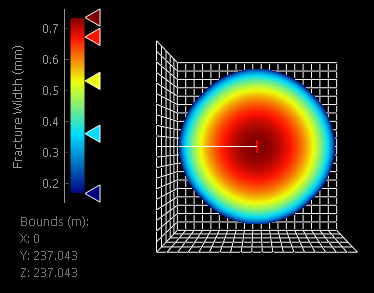
Figure 15: 3D KGD penny-shaped fracture width

Note

Here, the fluid loss effect, e.g. the fluid leakoff, is excluded because the governing equation is no longer self-similar when it is considered, so that an analytical approximation can hardly be obtained unless some other restrictions are applied, for example the uniform pressure distribution along the fracture in the toughness-dominated regime [6]. Thus, the leakoff is going to be introduced in the PKN Hydraulic Fracturing Model, another well known 2D classical hydraulic model.

[1]	Detournay: Propagation Regimes of Fluid-Driven Fractures in Impermeable Rocks. Int. J. Geomech., 4(1), 1-11 (2004)

[2]	(1, 2, 3, 4, 5, 6) Geertsma, de Klerk: A Rapid Method of Predicting Width and Extent of Hydraulically Induced Fractures. JPT 246, 1571-1581 (1969)

[3]	(1, 2, 3, 4, 5, 6) Savitski, Detournay: Propagation of a penny-shaped fluid-driven fracture in an impermeable rock: asymptotic solutions. IJSS 39, 6311-6337 (2002)

[4]	Adachi, Peirce: Asymptotic analysis of an elasticity equation for a finger-like hydraulic fracture, J. Elast. 90(1), 43-69 (2007)

[5]	Valko, Economides: Hydraulic Fracture Mechanics. Wiley, Chichester, UK (1995)

[6]	Bunger, Detournay, etc.: Toughness-dominated hydraulic fracture with leak-off. IJF 134, 175-190 (2005)