The derivation of Ramey solution
The Laplace transformation applied on Ramey solution
The subsidiary equation obtained with Laplace transformation
Ramey simplifies the wellbore heat transfer problem in cylindrical coordinate ( see here ) by mainly assuming:
- The steady heat flow for \(0 \le r \le r_w\) ;
- Heat conduction is only radial
Consequently, the transient heat conduction part for \(r>r_w\) can be derived from the transient heat transfer problem with three basic different boundary condition (BC) and initial condition (IC) as here in the region bounded internally by the circular cylinder \(r=r_w\).
The governing equation is:
And the initial condition is:
\(f(r)\) is a known function of \(r\) only. Apply the Laplace transformation on Eqn (1):
Using the theorems , we can get:
Initial temperature zero and constant temperature \(T_0\) at \(r=r_w\)
Eqn (4) is called the subsidiary equation, and \(q^2=\frac{s}{\kappa}\). In addition, Eqn (4) is a modified Bessel equation of zero order (see here) when \(f(r)=0\) .
The constant temperature boundary condition changes to Eqn (5) after the Laplace transformation:
And \(\bar{T}\) must be finite as \(r\rightarrow \infty\). Of the two solutions \(I_0(qr)\) and \(K_0(qr)\) (see here), the former \(I_0(qr)\) tends to infinity as \(r\rightarrow \infty\) and hence must be excluded. Thus, the solution is in terms of \(K_0(qr)\) and can be obtained as (see here for procedures):
Using the inversion theorem with \(s\) replaced by \(\lambda\) :
where: \(\mu = \sqrt{ \frac{\lambda}{\kappa} }\)
The integrand of Eqn (7) has a branch point at \(\lambda=0\) so that the contour of integral \((b)\) should be used. Because there is no zeros of \(K_0(\mu r)\) so that the contour integral Eqn (7) may be replaced by the sum of the integrals over \(CD\), \(EF\) and the small circle about the origin, which gives \(2 \pi i\) in the limit as its radius \(R \rightarrow 0\). And the final result is given as:
The heat flux \(q''\) across the wellbore/formation interface links the “outside” transient heat transfer and the “inside” steady one, thus \(q''\) obtained from Eqn (9) is of great importance and gives the derivation of the time function \(f(t)\) in the Ramey solution, which will be given later.
Constant initial temperature \(T_0\) and radiation at \(r=r_w\) into a medium at zero temperature
The subsidiary equation is:
And the boundary condition is:
Thus,
And:
The integrand of Eqn (13) has a branch point at \(\lambda=0\) so that the contour of integral \((b)\) should be used. Again, there are no poles within or on the contour. Following similar procedures, the final result is obtained as:
And the heat flux across the wellbore/formation interface is:
Initial temperature zero and constant flux \(q_0''\) at \(r=r_w\)
The similar procedure gives:
Notice that \(q\) is defined as \(q^2=\frac{s}{\kappa}\) here.
From the procedure presented here , the temperature solution for constant het flux \(q_0''\) is then given for large \(t_D=\frac{\kappa t}{r_w^2}\):
where: \(\ln c = 0.5722\) is known as Euler’s constant;
Note
For the details , user can check Chapter 13 in Ref.1 [1] .
The time function \(f(t)\) in Ramey solution
The time function \(f(t)\) of Ramey solution for any boundary condition is defined as:
where:
- \(dQ\) is the total heat flow across the interface of the differential element as shown in Fig 1 ;
- \(T_2, T_e\) represent the unknown formation temperature and the known earth temperature, respectively, i.e. \(T_2(r,0)=T_2(\infty,t)=T_e\) ;
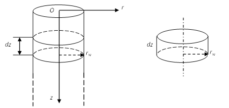
Figure 1: The differential element of the wellbore
If constant heat flux \(q_0''\) is assumed for the boundary condition at the interface \(r=r_w\), \(dQ=q_0''2\pi r_w dz\) and \(T_2-T_e\) equals to the solution \(T\) obtained as in Eqn (17), because the initial temperature is set to zero (\(T_2(r,0)=T_e\)). Thus, \(f(t)\) for constant heat flux \(q_0''\) and large dimensionless time \(t_D\) (\(t_D \geqslant 0.02\)) is:
Eqn (19) is exactly the expression of \(f(t)\) labeled as \((5)\) in Ramey’s paper [2] . And the constant \(-0.29\) comes from the Euler’s constant.
In other boundary conditions, the closed-form expression of \(f(t)\) is not available but can be obtained by evaluating the integrals numerically or making asymptotic expansions (user may check Chapter 13 in Ref.1 [1] for details ). As a consequence, the results of \(f(t)\) in the three boundary conditions (constant interface temperature, radiation at the interface, and the constant interface heat flux) are illustrated in the figure.
The Ramey solution [2]
A schematic view of wellbore heat transfer and the differential element for the Ramey solution is illustrated in Figure 2 :
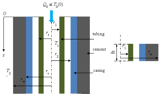
Figure 2: A schematic view of the wellbore heat transfer for Ramey solution and the differential element
The main assumption is as follows:
- The formation is homogeneous and isotropic;
- The properties of the fluid and formation are constant;
- Fluid in the tube flows with a constant mass flow rate \(W\) in the direction of the wellbore only;
- The heat conduction in the system is only radial;
- Steady radial heat flow is assumed inside the wellbore-formation interface (\(0 \leqslant r \leqslant r_w\)), hence it can be represented by a single steady-state heat transfer coefficient \(U\). [2] [3] ;
- The fluid temperature inside the tubing is lumped radially (\(T_1\) is the same for for \(0 \leqslant r \leqslant r_1\) at the same \(z\)) so that \(T_1\) is only the function of \(z\) and \(t\) : \(T_1(z,t)\);
- The initial formation temperature distribution is a known function of depth \(T_e(z)\) (initial condition);
- The temperature at far away satisfies the known function \(T_e(z)\) ( boundary condition);
- The surface fluid temperature is kept at \(T_0\).
With these assumptions, the energy balance for a differential element (\(0 \leqslant r \leqslant r_w\)), i.e. the rate of heat loss by fluid equals to the one transferred to the casing, yields:
where:
- \(c\) is the fluid heat capacity;
- \(T_2\) is the formation temperature.
In addition, according to Eqn (18), the rate of heat conduction from casing to surrounding formation is:
Therefore:
Substitution Eqn (23) into Eqn (20):
where: the function \(A\) is:
Assuming linear geothermal gradient: \(T_e = az+b\):
An integral factor for Eqn (26) is \(e^{\frac{z}{A}}\):
Thus:
The function \(C(t)\) may be evaluated from the condition that \(T_1=T_0\) for \(z=0\), thus:
And the final expression for Ramey solution is:
| [1] | (1, 2) Carslaw and Jaeger: Conduction of Heat in Solids, 2nd edition. Oxford University Press, Oxford, UK (1959) |
| [2] | (1, 2, 3) Ramey: Wellbore heat transmission, JPT, 427-435 (April 1962) |
| [3] | Moradi, Awang: Heat transfer in the formation, SPE, 6 (21), 3927-3932 (2013) |