Separation of variables
Consider a partial differential equation (PDE) of the diffusion type:
(1)\[\frac{\partial u}{\partial t} = \alpha^2 \frac{\partial^2 u}{\partial x^2},
\ \ \ \ 0<x<L,\ \ 0<t<\infty\]
with the boundary conditions (BCs):
(2)\[\begin{split}\left\{
\begin{align}
& u(0,t) = 0 \\
& u(L,t) = 0 \\
\end{align}
\right.\end{split}\]
and the initial condition (IC):
(3)\[u(x,0) = \varphi(x), \ \ \ \ 0 \leqslant x \leqslant L\]
where:
- \(\alpha\) and \(L\) are both known constants;
- \(\varphi(x)\) is a known function of \(x\) only.
The separation of variables looks for simple-type solutions to the PDE of
the form:
(4)\[u(x,t) = X(x) \bullet T(t)\]
where:
- \(X\) is some function of \(x\);
- \(T\) is some function of \(t\).
The general idea is that it is possible to find an infinite number of these
solutions to the PDE. These simple solutions called fundamental solutions of
the form: \(u_n=X_n(x) \bullet T_n(t)\) are the building blocks of the
problem. Thus, the solution \(u(x,t)\) is found by adding those
fundamental solutions:
\[u=\sum_{n=1}^\infty A_nX_n(x)\bullet T_n(t),\]
where
- \(A_n\) are the constants determined by BCs and IC;
- \(n\) is a natural number.
Then the following procedures will find out the solutions \(u(x,t)\):
Finding the elementary solutions
With the definition:
(5)\[\begin{split}\left\{
\begin{align}
& \dot{u} = \frac{\partial u}{\partial t} \\
& u' = \frac{\partial u}{\partial x} \\
& u'' = \frac{\partial^2 u}{\partial x^2} \\
\end{align}
\right.\end{split}\]
Eqn (1) can be written as:
\[X\dot{T} = \alpha^2 TX''\]
Divide each side by \(\alpha^2 XT\), the separated variables are obtained:
(6)\[\frac{\dot{T}}{\alpha^2 T} = \frac{X''}{X}\]
The left side of Eqn (6) depends only on \(t\) and the right
side depends only on on \(x\) . Because \(x\) and \(t\) are
independent of each other, each side must equal to a constant \(k\) :
\[\frac{\dot{T}}{\alpha^2 T} = \frac{X''}{X} = k\]
or
(7)\[\begin{split}\left\{
\begin{align}
& \dot{T} -k\alpha^2 T = 0 \\
& X''-kX = 0 \\
\end{align}
\right.\end{split}\]
Now the PDE has been reduced to two ODEs of standard-type which have the
solutions:
(8)\[T = C_1e^{k\alpha^2t}\]
Observation on Eqn (8) indicates that the separated constant \(k\)
needs to be negative otherwise \(T\) does not go zero when
\(t \rightarrow \infty\) as in the Eqn (2). Therefore:
(9)\[k = -\lambda^2\]
where: \(\lambda\) is a nonzero real number.
Then the solution to the ODEs as Eqn (7) are:
(10)\[\begin{split}\left\{
\begin{align}
& T = C_1e^{-\lambda^2 \alpha^2 t} \\
& X = C_2 \sin(\lambda x) + C_3 \cos(\lambda x) \\
\end{align}
\right.\end{split}\]
Consequently, the fundamental solution is of the form:
(11)\[u_n = X_n(x)\bullet T_n(t) = e^{-\lambda^2 \alpha^2 t}
[A_n \sin(\lambda x) + B_n \cos(\lambda x)]\]
The \(A_n\), \(B_n\) and \(C\) are all arbitrary constants.
Determine the constants \(\lambda, A\) and \(B\) with the BCs and IC
The constants \(\lambda, A\) and \(B\) in the elementary solutions
(Eqn (11)) can be determined by BCs and IC. First the BCs
are considered:
(12)\[\begin{split}\left\{
\begin{align}
& u_n(0,t) = B_ne^{-\lambda^2 \alpha^2 t} = 0 \Rightarrow B_n=0 \\
& u_n(L,t) = A_ne^{-\lambda^2 \alpha^2 t} \sin(\lambda L) = 0
\Rightarrow \sin(\lambda L)=0\\
\end{align}
\right.\end{split}\]
Because \(\lambda \neq 0\), Eqn (12) makes:
(13)\[\lambda = \pm\frac{\pi}{L}, \ \pm\frac{2\pi}{L}, \ \pm\frac{3\pi}{L}, ...\]
or
(14)\[\lambda_n = \pm\frac{n\pi}{L}\]
Therefore, the fundamental solutions are of the form:
(15)\[u_n = A_n e^{ -( {\frac{n\pi}{L}\alpha} )^2 t } \sin(\frac{n\pi}{L}x)\]
And the solution to the PDE is:
(16)\[u = \sum_{n=1}^\infty A_n e^{ -( {\frac{n\pi}{L}\alpha} )^2 t } \sin
(\frac{n\pi}{L}x)\]
The remaining constants \(A_n\) can be determined with the IC:
\(u(x,0) = \varphi(x)\) .
Substitute Eqn (16) into the IC:
(17)\[\varphi(x) = \sum_{n=1}^\infty A_n \sin(\frac{n\pi}{L}x)\]
As long as \(\varphi(x)\) is continuous, it can be expanded in the form
known as the half sine expansion as in Eqn (17) . Notice that the
function \(\sin(\frac{n\pi}{L}x)\) is orthogonal:
(18)\[\begin{split}\begin{equation}
\begin{split}
I& = \int_0^L \sin\frac{m\pi}{L}x \sin\frac{n\pi}{L}xdx \\
& = \frac{1}{2} \int_0^L [ \cos(\frac{m-n}{L}\pi x)
-\cos(\frac{m+n}{L}\pi x) ] dx \\
& = \left\{ \begin{array}{ll}
\frac{1}{2}[ \frac{L}{(m-n)\pi}\sin(\frac{m-n}{L}\pi x) -
\frac{L}{(m+n)\pi}\sin(\frac{m+n}{L}\pi x)]
\vert_0^L & m \neq n \\
\frac{1}{2}[ 1 -\frac{L}{(m+n)\pi}\sin(\frac{m+n}{L}\pi x)]
\vert_0^L & m = n \\
\end{array} \right. \\
& = \left\{ \begin{array}{ll}
0 & m \neq n \\
\frac{L}{2} & m = n \\
\end{array} \right.
\end{split}
\end{equation}\end{split}\]
where: \(m\) is an arbitrary integer.
Then we multiply Eqn (17) by \(\frac{\sin(n\pi x)}{L}\) ,
integrate from \(0\) to \(L\) and drop out all the zero terms due to
orthogonality:
(19)\[\begin{split}\begin{equation}
\begin{split}
\int_0^L \varphi(x) \sin(\frac{n\pi}{L}x)dx& = A_n \int_0^L
\sin^2(\frac{n\pi}{L}x)dx \\
& = \frac{L}{2}A_n \\
\end{split}
\end{equation}\end{split}\]
Hence:
(20)\[A_n = \int_0^L \varphi(x) \sin(\frac{n\pi}{L}x)dx\]
Having reached here, we can write down the solution \(u(x,t)\) as:
(21)\[u = \sum_{n=1}^\infty A_n e^{ -( {\frac{n\pi}{L}\alpha} )^2 t } \sin
(\frac{n\pi}{L}x)\]
with the coefficients \(A_n\) defined in Eqn (20) .
Note
The separation of variables method is only applicable for the
homogeneous diffusion-type PDE with homogeneous BCs. When the
BCs is not homogeneous, they need to be transformed to homogeneous ones
before the separation of variables method is implemented.
Transforming the nonhomogeneous BCs into the homogeneous ones
Transforming method
This section mainly consider the boundary conditions as constants.
Consider a partial differential equation (PDE) of the diffusion type:
(22)\[\frac{\partial u}{\partial t} = \alpha^2 \frac{\partial^2 u}{\partial x^2},
\ \ \ \ 0<x<L,\ \ 0<t<\infty\]
with the boundary conditions (BCs):
(23)\[\begin{split}\left\{
\begin{align}
& u(0,t) = u_1 \\
& u(L,t) = u_2 \\
\end{align}
\right.\end{split}\]
and the initial condition (IC):
(24)\[u(x,0) = \varphi(x), \ \ \ \ 0 \leqslant x \leqslant L\]
where:
- \(\alpha\) , \(L\) , \(u_1\) and \(u_2\) are all known
constants;
- \(\varphi(x)\) is a known function of \(x\) only.
Comparing the problem to the one in the previous section, the BCs become non-
homogeneous so that the separation of variables cannot be applied directly here.
However, if the nonhomogeneous BCs can be transformed to homogeneous ones,
the method becomes applicable.
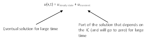
The solution based on the separated variables
as in Eqn (21) is found to have a steady-state solution (solution
when \(t \rightarrow \infty\)) as \(0\) . Then,
it seems reasonable to treat the solution \(u\) for Eqn (22) with
conditions Eqn (23) and Eqn (24) as the sum of the two parts
as shown in :
In mathematical form:
(25)\[u = [u_1 + \frac{x}{L}(u_2-u_1)] + U(x,t)\]
where: \(U(x,t)\) represents the transient part of the solution.
Substitute Eqn (25) into the original problem:
(26)\[\frac{\partial U}{\partial t} = \alpha^2 \frac{\partial^2 U}{\partial x^2},
\ \ \ \ 0<x<L,\ \ 0<t<\infty\]
with the new boundary conditions (BCs):
(27)\[\begin{split}\left\{
\begin{align}
& U(0,t) = 0 \\
& U(L,t) = 0 \\
\end{align}
\right.\end{split}\]
and the new initial condition (IC):
(28)\[\begin{split}\begin{equation}
\begin{split}
U(x,0)&= \bar{\varphi}(x) \\
&= \varphi(x)-[u_1 + \frac{x}{L}(u_2-u_1)], \ \ \ 0 \leqslant x \leqslant L
\end{split}
\end{equation}\end{split}\]
where: \(\bar{\varphi}(x)\) denotes the new IC.
Then the new set of the PDE associated with the new BCs and IC can
be solved with separated variables :
(29)\[U = \sum_{n=1}^\infty A_n e^{ -( {\frac{n\pi}{L}\alpha} )^2 t } \sin
(\frac{n\pi}{L}x)\]
with the coefficients \(A_n\) as:
(30)\[A_n = \int_0^L \bar{\varphi}(x) \sin(\frac{n\pi}{L}x)dx\]
Constant IC
When the IC is also a constant, \(\varphi(x)=u_0\) :
(31)\[\begin{split}\begin{equation}
\begin{split}
A_n&= \frac{2}{L} \int_0^L [ u_0-u_1 - \frac{x}{L}(u_2-u_1) ]
\sin(\frac{n\pi}{L}x)dx \\
&= \frac{2(u_0-u_1)}{L}\int_0^L \sin(\frac{n\pi}{L}x)dx
+ \frac{2(u_1-u_2)}{L}\int_0^L \frac{x}{L} \sin(\frac{n\pi}{L}x)dx \\
&= \frac{2(u_0-u_1)}{L} \frac{-L}{n\pi}\cos(\frac{n\pi}{L}x) \vert_0^L +
\frac{2(u_1-u_2)}{(n\pi)^2}
\int_0^L \frac{n\pi x}{L}\sin(\frac{n\pi x}{L})d{\frac{n\pi x}{L}}
\end{split}
\end{equation}\end{split}\]
Define \(\xi = \frac{n\pi}{L}x\), \(\xi \in [0,n\pi]\):
(32)\[\begin{split}\begin{equation}
\begin{split}
A_n&= \frac{2(u_0-u_1)}{n\pi} \cos(\frac{n\pi}{L}x)\vert_L^0 +
\frac{2(u_1-u_2)}{(n\pi)^2} \int_0^{n\pi} \xi \sin\xi d\xi \\
&= \frac{2(u_0-u_1)}{n\pi}(1-\cos n\pi) +
\frac{2(u_1-u_2)}{(n\pi)^2} (\sin\xi - \xi\cos\xi)\vert_0^{n\pi} \\
&= \frac{2(u_0-u_1)}{n\pi}(1-\cos n\pi) -
\frac{2(u_1-u_2)}{(n\pi)^2} n\pi \cos n\pi \\
&= \frac{2}{n\pi} [ (u_0-u_1)(1-\cos n\pi) - (u_1-u_2)\cos n\pi ] \\
\end{split}
\end{equation}\end{split}\]
Therefore:
(33)\[\begin{split}A_n = \left\{ \begin{array}{ll}
\frac{2(u_2-u_1)}{n\pi} & \textrm{n is even} \\
\frac{2}{n\pi}(2u_0-u_1-u_2) & \textrm{n is odd} \\
\end{array} \right.\end{split}\]
Similarity solution
When the boundary condition (BCs) Eqn (2) becomes unbounded,
i.e. one of the BCs takes \(x \rightarrow \infty\):
(34)\[\begin{split}\left\{
\begin{align}
& u(0,t) = u_c \\
& u(\infty,t) = u_0 \\
\end{align}
\right.\end{split}\]
where: \(u_c\) and \(u_0\) are both known constants.
A special method called “similarity solution” is derived to solve the
PDE associated with this type of BCs.
Usually, the boundary condition at the infinity equals to the initial
condition because the change due to physical mechanisms (for example,
the diffusion phenomena ) will not affect the remote medium. Thus, the PDE
is:
(35)\[\frac{\partial u}{\partial t} = \alpha^2 \frac{\partial^2 u}{\partial x^2},
\ \ \ \ 0<x<\infty,\ \ 0<t<\infty\]
associated with the BCs as Eqn (34) and the IC:
(36)\[u(x,0) = u_0, \ \ \ \ x \geqslant L\]
Reduction PDE to ODE
First, the dilation transformation is carried on \(x\) and \(t\) so
that a couple of new variables \(z\) and \(s\) are obtained:
(37)\[\begin{split}\left\{
\begin{align}
& z = \epsilon^a x \\
& s = \epsilon^b t \\
\end{align}
\right.\end{split}\]
Consequently, a new function \(p\) is obtained such that:
(38)\[p(z,s) = \epsilon^c u( \epsilon^{-a}z, \epsilon^{-b}s )\]
where: \(a\) , \(b\) , \(c\) and \(\epsilon\) are arbitrary
constants.
Then, notice that \(\frac{\partial^2 z}{\partial x^2} = 0\), we have :
(39)\[\begin{split}\left\{
\begin{align}
& \frac{\partial u}{\partial t} = \epsilon^{-c} \frac{\partial p}
{\partial s} \frac{\partial s}{\partial t}
=\epsilon^{b-c} \frac{\partial p}{\partial s} \\
& \frac{\partial^2 u}{\partial x^2} = \epsilon^{-c} \frac{\partial^2 p}
{\partial x^2}
=\epsilon^{-c}[ \frac{\partial^2 p}{\partial z^2}
(\frac{\partial z}{\partial x})^2 +
\frac{\partial p}{\partial z}\frac{\partial^2
z}{\partial x^2} ]
= \epsilon^{2a-c} \frac{\partial^2 p}{\partial z^2} \\
\end{align}
\right.\end{split}\]
Thus, the original PDE Eqn (35) becomes:
(40)\[\epsilon^{b-c} \frac{\partial p}{\partial s}
= \epsilon^{2a-c} \alpha^2 \frac{\partial^2 p}{\partial z^2}\]
The PDE becomes invariant under the transformation Eqn (37) and
Eqn (38) if \(b-c=2a-c\), i.e. \(b=2a\) . That means
\(u(x,t)\) solves Eqn (35) in the variables \(x,t\) while
\(p(z,s)\) solves the same equation in the variables \(z,s\) ,
and the two groups of variables satisfies according to \(b=2a\) .
(41)\[\frac{x}{\sqrt{t}} = \frac{z}{\sqrt{s}}\]
Therefore, the PDE can be reduced to an ODE (cancel \(x\) or
\(t\) so that the number of independent arguments is reduced from
\(2\) to \(1\)) by introducing \(\xi = \frac{x}{\sqrt{t}}\) ,
known as the Boltzmann transformation.
In addition, we have:
(42)\[ps^{-\frac{c}{b}}=(\epsilon^c u)(\epsilon^b t)^{-\frac{c}{b}}=ut^{-\frac{c}{b}}\]
Therefore, we can introduce with \(b=2a\):
(43)\[u=t^{\frac{c}{b}}y(\xi)=t^{\frac{c}{2a}}y(\xi)\]
where: \(y\) is the function of \(\xi\) only.
Then, we have:
(44)\[\begin{split}\begin{equation}
\begin{split}
\frac{\partial u}{\partial t}&= \frac{c}{2a}t^{\frac{c}{2a}-1}y(\xi) +
t^{\frac{c}{2a}}
\frac{\partial y}{\partial \xi}
\frac{\partial \xi}{\partial t} \\
&= \frac{c}{2a}t^{\frac{c}{2a}-1}y(\xi) +
t^{\frac{c}{2a}}(-\frac{1}{2}xt^{-\frac{3}{2}})
\frac{\partial y}{\partial \xi} \\
&\stackrel{\xi=xt^{-\frac{1}{2}}}= \frac{c}{2a}
t^{\frac{c}{2a}-1}y(\xi) +
t^{\frac{c}{2a}-1}(-\frac{\xi}{2})
\frac{\partial y}{\partial \xi} \\
&= t^{\frac{c}{2a}-1}[ \frac{c}{2a}y(\xi) -
\frac{\xi}{2} \frac{\partial y}
{\partial \xi}]
\end{split}
\end{equation}\end{split}\]
And:
(45)\[\frac{\partial u}{\partial x}=t^{\frac{c}{2a}}\frac{\partial y}{\partial
\xi} \frac{\partial \xi}{\partial x}
= t^{\frac{c-a}{2a}}\frac{\partial y}{\partial \xi}\]
(46)\[\begin{split}\begin{equation}
\begin{split}
\frac{\partial u^2}{\partial x^2}&= \frac{\partial}{\partial x}
(t^{\frac{c-a}{2a}}\frac{\partial y}{\partial \xi} ) \\
&= t^{\frac{c-a}{2a}}\frac{\partial}
{\partial \xi}(\frac{\partial y}{\partial \xi})\frac
{\partial \xi}{\partial x} \\
&= t^{\frac{c}{2a}-1}\frac
{\partial^2 y}{\partial \xi^2} \\
\end{split}
\end{equation}\end{split}\]
Combination of Eqn (44) , Eqn (46) and the PDE Eqn
(35) by cancelling term \(t^{\frac{c}{2a}-1}\) yields the new PDE:
(47)\[\alpha^2 \frac{\partial^2 y}{\partial \xi^2} +
\frac{\xi}{2}\frac{\partial y}{\partial \xi} - \frac{c}{2a}y(\xi)=0\]
Because \(y\) is the function of \(\xi\) only, the PDE Eqn
(47) can be rewritten as an ODE:
(48)\[\alpha^2 \frac{d^2 y}{d \xi^2} +
\frac{\xi}{2}\frac{d y}{d \xi} - \frac{c}{2a}y(\xi)=0\]
The ODE Eqn (48) is the new ODE obtained from the original PDE
Eqn (35) and the new unknown function \(y(\xi)\) is what needs
solving by methods that can be used to solve ODE.
The solution
The boundary condition after the previous transformation
\(u(0,t) = t^{\frac{c}{2a}}y(0)\) can equal to the constant \(u_c\)
if and only if \(c=0\) . In this case, the equation Eqn (48) is
further reduced to:
(49)\[\alpha^2 \frac{d^2 y}{d \xi^2} + \frac{\xi}{2}\frac{d y}{d \xi} =0\]
With the BCs:
(50)\[\begin{split}\left\{
\begin{align}
& y(0) = u_c \\
& y(\infty)=u_0 \\
\end{align}
\right.\end{split}\]
Notice that the transformation \(\xi = \frac{x}{\sqrt{t}}\) makes
\(\xi\) approaches the infinity either \(x \rightarrow \infty\) or
\(t=0\) . Thus, the original boundary condition at \(x \rightarrow
\infty\) and the original initial condition at \(t=0\) are unified to
\(\xi \rightarrow \infty\). Then the original BCs and IC are
said to be self-similar on such a condition.
Integration on Eqn (49) yields:
(51)\[\frac{dy}{d\xi} = C_1e^{\frac{\xi^2}{4\alpha^2}}\]
Integration on Eqn (51) obtains:
(52)\[\begin{split}\begin{equation}
\begin{split}
y(\xi)&= C_1\int_0^\xi e^{-\frac{\lambda^2}{4\alpha^2}}d\lambda + C_2 \\
&= C_3 \textrm{erf}(\frac{\xi}{2\alpha}) + C_2
\end{split}
\end{equation}\end{split}\]
where:
- \(\textrm{erf}(z)=\frac{2}{\sqrt{\pi}}\int_0^ze^{-\eta^2}d\eta\) is known as
error function and \(\textrm{erf}(0)=0\), \(\textrm{erf}(\infty)=1\);
- \(\lambda\) and \(\eta\) are both dummy integral variables;
- \(Cs\) are all arbitrary constants determined by BCs
Apply \(y(0) = u_c\) and \(y(\infty)=u_0\), we have:
(53)\[\begin{split}\left\{
\begin{align}
& C_2 = u_c \\
& C_3=u_0-u_c \\
\end{align}
\right.\end{split}\]
Then the function \(y\) is solved as:
(54)\[\begin{split}\begin{equation}
\begin{split}
y(\xi)&= (u_0-u_c)\textrm{erf}(\frac{\xi}{2\alpha})+u_c \\
&= (u_c-u_0)\textrm{erfc}(\frac{\xi}{2\alpha})+u_0 \\
\end{split}
\end{equation}\end{split}\]
where: \(\textrm{erfc}(z)=1-\textrm{erf}(z)\) .
Because \(c=0\) and \(\xi = \frac{x}{\sqrt{t}}\) ,
the original solution to
the PDE Eqn (35)
associated with the BCs Eqn (34) and the IC Eqn (36)
is:
(55)\[\begin{split}\begin{equation}
\begin{split}
u(x,t)&= t^{\frac{c}{2a}}y(\xi) \\
&= y(\xi) \\
&= (u_c-u_0)\textrm{erfc}(\frac{x}{2\alpha \sqrt{t}})+u_0 \\
\end{split}
\end{equation}\end{split}\]