Introduction
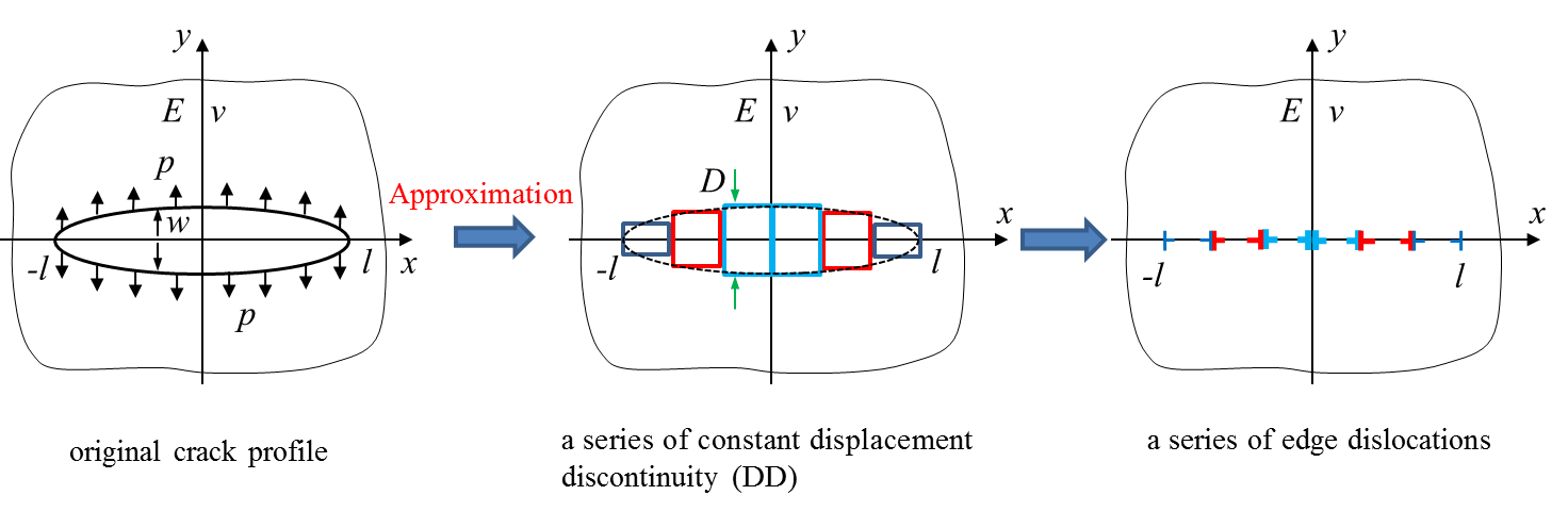
The displacement discontinuity method (DDM) uses the physical analog of a
slit-like crack and a series of distribution of dislocations
(). Consequently, it only needs to discretize
the crack surfaces, making itself perhaps the most efficient method for
crack problems . The DDM is applied for crack problems based on the
fundamental dislocation theory.
\(E\) and \(v\) represent the Young’s modulus and Poisson ratio.
Fundamental dislocation theory in DDM
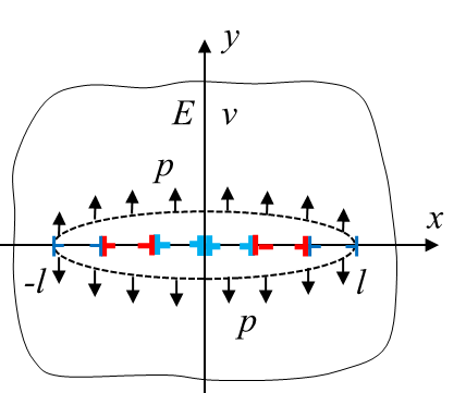
The DDM uses the physical analog of a slit-like crack and a series distribution
of edge dislocation dipoles in a homogeneous medium ().
Each dipole represents a crack element and a constant opening over it.
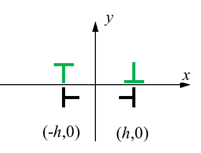
The stress components due to two pairs of dislocation dipoles (
) are:
(1)\[\begin{split}\left\{
\begin{align}
& \sigma_{yy} = b_x k y(A_4-A_3) + b_y k [(x+h)A_6 - (x-h)A_5] \\
& \sigma_{xy} = b_x k [(x+h)A_4 - (x-h)A_3] + b_y k y(A_4-A_3) \\
\end{align}
\right.\end{split}\]
where,
(2)\[\begin{split}\left\{
\begin{align}
& A_3 = \frac{(x-h)^2-y^2}{ \big[(x-h)^2+y^2 \big]^2 } \\
& A_4 = \frac{(x+h)^2-y^2}{ \big[(x+h)^2+y^2 \big]^2 } \\
& A_5 = \frac{(x-h)^2+3y^2}{ \big[(x-h)^2+y^2 \big]^2 } \\
& A_6 = \frac{(x+h)^2+3y^2}{ \big[(x+h)^2+y^2 \big]^2 } \\
\end{align}
\right.\end{split}\]
and
(3)\[k = \frac{G}{2\pi(1-v)}\]
and \(G\) is the shear modulus.
The \(b_x\) and \(b_y\) are the burger’s vectors analog to the
constant shear opening \(D_x\) and normal opening \(D_y\) over a
crack element, respectively.
Influence coefficients
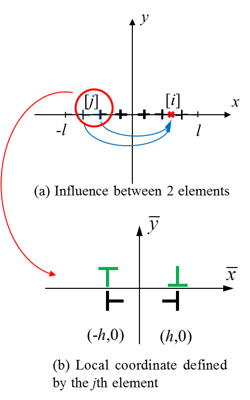
Influence between two elements
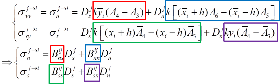
The influence between two crack elements, say the stress at the center of the
\(i\) th element (field element) due to the dislocation dipole pairs
over the \(j\) th element (source element), is illustrated in
(a)
and calculated as :
where,
(4)\[\begin{split}\left\{
\begin{align}
& \bar {A_3} = \frac{(\bar x_i-h)^2-\bar y_i^2}{ \big[(\bar x_i-h)^2+\bar y_i^2 \big]^2 } \\
& \bar {A_4} = \frac{(\bar x_i+h)^2-\bar y_i^2}{ \big[(\bar x_i+h)^2+\bar y_i^2 \big]^2 } \\
& \bar {A_5} = \frac{(\bar x_i-h)^2+3\bar y_i^2}{ \big[(\bar x_i-h)^2+\bar y_i^2 \big]^2 } \\
& \bar {A_6} = \frac{(\bar x_i+h)^2+3\bar y_i^2}{ \big[(\bar x_i+h)^2+\bar y_i^2 \big]^2 } \\
\end{align}
\right.\end{split}\]
and,
- \((\bar x_i, \bar y_i)\) are the center coordinate of the \(i\) th
element under the local coordinate defined by the \(j\) th element (
(b))
- \(h\) is the half size of the \(j\) th element
- The coefficients \(B\) etc. are the influence coefficients.
Note
From Eqn (4), the influence between two elements is proportional to
\(r^{-2}\), where \(r\) represents the distance between the two
elements.
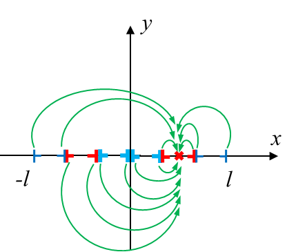
The total influence on an element
Then the stress at the center of the field (\(i\) th) element due to
all the dislocation dipoles (say \(N\) source elements,
as illustrated in ) over the crack surface
is obtained as Eqn (6):
(5)\[\begin{split}\left\{
\begin{align}
& \sigma _n^i = \sum_{j=1}^NB_{ns}^{ij} D_s^j +
\sum_{j=1}^NB_{nn}^{ij} D_n^j = p_n^i\\
& \sigma _s^i = \sum_{j=1}^NB_{ss}^{ij} D_s^j +
\sum_{j=1}^NB_{sn}^{ij} D_n^j = p_s^i\\
\end{align} \\
\Downarrow
\right.\end{split}\]
(6)\[\begin{split}\left\{
\begin{align}
& \sum_{j=1}^NB_{ns}^{ij} D_s^j + \sum_{j=1}^NB_{nn}^{ij} D_n^j = p_n^i\\
& \sum_{j=1}^NB_{ss}^{ij} D_s^j + \sum_{j=1}^NB_{sn}^{ij} D_n^j = p_s^i\\
\end{align}
\right.\end{split}\]
where,
- \(p_s^i\) and \(p_n^i\) are the shear and normal tractions
applied on the field (\(i\) th) element.
- \(D_s^i\) and \(D_n^i\) are the shear and normal openings
(displacement discontinuities) over the field (\(i\) th) element.
Coefficient matrix
The coefficient matrix is assembled by ranging the index of the field
(\(i\) th)element from \(1\) to \(N\).
(7)\[\begin{split}\left[ \begin{array}{ccc}
{B}_{ss}^{11} & {B}_{sn}^{11} & \ldots & \ldots &
{B}_{ss}^{1j} & {B}_{sn}^{1j} & \ldots & \ldots &
{B}_{ss}^{1N} & {B}_{sn}^{1N} \\
{B}_{ns}^{11} & {B}_{nn}^{11} & \ldots & \ldots &
{B}_{ns}^{1j} & {B}_{nn}^{1j} & \ldots & \ldots &
{B}_{ns}^{1N} & {B}_{nn}^{1N} \\
\vdots & \vdots & \ddots & \ddots &
\vdots & \vdots & \ddots & \ddots &
\vdots & \vdots \\
\vdots & \vdots & \ddots & \ddots &
\vdots & \vdots & \ddots & \ddots &
\vdots & \vdots \\
{B}_{ss}^{i1} & {B}_{sn}^{i1} & \ldots & \ldots &
{B}_{ss}^{ij} & {B}_{sn}^{ij} & \ldots & \ldots &
{B}_{ss}^{iN} & {B}_{sn}^{iN} \\
{B}_{ns}^{i1} & {B}_{nn}^{i1} & \ldots & \ldots &
{B}_{ns}^{ij} & {B}_{nn}^{ij} & \ldots & \ldots &
{B}_{ns}^{iN} & {B}_{nn}^{iN} \\
\vdots & \vdots & \ddots & \ddots &
\vdots & \vdots & \ddots & \ddots &
\vdots & \vdots \\
\vdots & \vdots & \ddots & \ddots &
\vdots & \vdots & \ddots & \ddots &
\vdots & \vdots \\
{B}_{ss}^{N1} & {B}_{sn}^{N1} & \ldots & \ldots &
{B}_{ss}^{Nj} & {B}_{sn}^{Nj} & \ldots & \ldots &
{B}_{ss}^{NN} & {B}_{sn}^{NN} \\
{B}_{ns}^{N1} & {B}_{nn}^{N1} & \ldots & \ldots &
{B}_{ns}^{Nj} & {B}_{nn}^{Nj} & \ldots & \ldots &
{B}_{ns}^{NN} & {B}_{nn}^{NN} \\
\end{array}
\right] \left[ \begin{array}{ccc}
D_s^1 \\
D_n^1 \\
\vdots \\
\vdots \\
D_s^j \\
D_n^j \\
\vdots \\
\vdots \\
D_s^N \\
D_n^N \\
\end{array}
\right] = \left[ \begin{array}{ccc}
p_s^1 \\
p_n^1 \\
\vdots \\
\vdots \\
p_s^i \\
p_n^i \\
\vdots \\
\vdots \\
p_s^N \\
p_n^N \\
\end{array}
\right]\end{split}\]
According to the Einstein notation, Eqn (7)
can be written in a more concise form:
(8)\[\mathbf{K}_{ij} \mathbf{D}_j = \mathbf{p}_i\]
where,
(9)\[ \begin{align}\begin{aligned}\begin{split}\mathbf{K}_{ij} = \left[ \begin{array}{ccc}
{B}_{ss}^{ij} & {B}_{sn}^{ij} \\
{B}_{ns}^{ij} & {B}_{nn}^{ij} \\
\end{array}
\right]\end{split}\\\begin{split}\mathbf{D}_j = \left[ \begin{array}{ccc}
D_s^j \\
D_n^j \\
\end{array}
\right]\end{split}\\\begin{split}\mathbf{p}_i = \left[ \begin{array}{ccc}
p_s^i \\
p_n^i \\
\end{array}
\right]\end{split}\end{aligned}\end{align} \]
Then, the crack opening is obtained by:
(10)\[\mathbf{D}_j = \mathbf{K}_{ij}^{-1} \mathbf{p}_i\]