Derivation of the Governing Equations of KGD and PKN model¶

Navier-Stokes (NS) equations¶

Cylindrical Coordinate¶

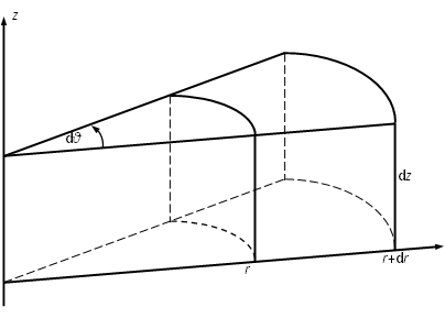
Figure 1: An infinitesimal element in Cylindrical coordinate

For the cylindrical coordinate as shown in Figure 1, the NS equation can be written as in scalar forms as Eqn (3):

(3)\[\begin{split}\left\{ \begin{align} & \rho (\frac{\partial u_r}{\partial t} + u_r\frac{\partial u_r}{\partial r} + \frac{u_\theta}{r}\frac{\partial u_r}{\partial \theta} - \frac{u^2_{\theta}}{r}+ u_z\frac{\partial u_r}{\partial z}) \\ & = -\frac{\partial p}{\partial r} + \mu[\frac{1}{r}\frac{\partial}{\partial r}(r\frac{\partial u_r}{\partial r}) + \frac{1}{r^2}\frac{\partial^2 u_r}{\partial \theta^2} + \frac{\partial^2 u_r}{\partial z^2} - \frac{u_r}{r^2} - \frac{2}{r^2}\frac{\partial u_\theta}{\partial \theta}] + \rho g_r \\ & \rho (\frac{\partial u_\theta}{\partial t} + u_r\frac{\partial u_\theta}{\partial r} + \frac{u_\theta}{r}\frac{\partial u_\theta}{\partial \theta} + u_z\frac{\partial u_\theta}{\partial z} + \frac{u_r u_\theta}{r}) \\ & = -\frac{1}{r}\frac{\partial p}{\partial \theta} + \mu[\frac{1}{r}\frac{\partial}{\partial r}(r\frac{\partial u_\theta}{\partial r}) + \frac{1}{r^2}\frac{\partial^2 u_\theta}{\partial \theta^2} + \frac{\partial^2 u_\theta}{\partial z^2} + \frac{2}{r^2}\frac{\partial u_r}{\partial \theta}] + \rho g_\theta \\ & \rho (\frac{\partial u_z}{\partial t} + u_r\frac{\partial u_z}{\partial r} + \frac{u_\theta}{r}\frac{\partial u_z}{\partial \theta} + u_z\frac{\partial u_z}{\partial z}) \\ & = -\frac{\partial p}{\partial z} + \mu[\frac{1}{r}\frac{\partial}{\partial r}(r\frac{\partial u_z}{\partial r}) + \frac{1}{r^2}\frac{\partial^2 u_z}{\partial \theta^2} + \frac{\partial^2 u_z}{\partial z^2} ] + \rho g_z \\ \end{align} \right.\end{split}\]

or in as Eqn (2) in tensor notation form with the subscripts \(i\) and \(j\) representing the coordinate components \(r\) , \(\theta\) and \(z\) instead of \(x\) , \(y\) and \(z\);

Special case: Axisymmetric flow without tangential velocity¶

A very common case for Cylindrical coordinate is axisymmetric flow (\(\frac{\partial}{\partial\theta}=0\)) without tangential velocity (\(u_\theta=0\) ). Then all the terms associated with \(\theta\) becomes zero and the NS equations Eqn (3) are reduced to Eqn (4):

(4)\[\begin{split}\left\{ \begin{align} & \rho (\frac{\partial u_r}{\partial t} + u_r\frac{\partial u_r}{\partial r} + u_z\frac{\partial u_r}{\partial z}) \\ & = -\frac{\partial p}{\partial r} + \mu[\frac{1}{r}\frac{\partial}{\partial r}(r\frac{\partial u_r}{\partial r}) + \frac{\partial^2 u_r}{\partial z^2} - \frac{u_r}{r^2} ] + \rho g_r \\ & \rho (\frac{\partial u_z}{\partial t} + u_r\frac{\partial u_z}{\partial r} + u_z\frac{\partial u_z}{\partial z}) \\ & = -\frac{\partial p}{\partial z} + \mu[\frac{1}{r}\frac{\partial}{\partial r}(r\frac{\partial u_z}{\partial r}) + \frac{\partial^2 u_z}{\partial z^2} ] + \rho g_z \\ \end{align} \right.\end{split}\]

Note

All the parameters in this document are with S.I. units unless specified.

Lubrication theory¶

Reynolds equation¶

A 3D hydraulic fracturing size is shown in Figure 2, in which the fluid is flowing inside a large chanel (tens to over hundreds of meters \(x\) and \(y\) directions) with a very narrow opening (the fracture width \(w\) measured in millimeters in \(z\) direction). Then the lubrication theory can be applied on the hydraulic fracturing model if the fluid is assumed an incompressible Newtonian laminar fluid.

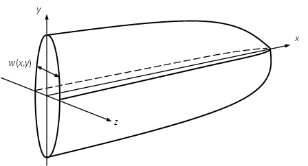
Figure 2: A 3D hydraulic fracture size

Cartesian coordinate¶

In the Cartesian coordinate the lubrication theory yields:

\[\begin{split}\left\{ \begin{align} & \frac{\partial p}{\partial x} = \mu\frac{\partial^2 u_x}{\partial z^2} \\ & \frac{\partial p}{\partial y} = \mu\frac{\partial^2 u_y}{\partial z^2} \\ \end{align} \right.\end{split}\]

Integration of the above equations with respect to \(z\) with the non-slip boundary conditions (5th assumption of the lubrication theory) for fracture width \(w(x,y,t)\) (zero velocity at \(\pm \frac{w}{2}\)) gives:

(11)\[\begin{split}\left\{ \begin{align} & u_x = -\frac{1}{2\mu}[\frac{w^2}{4}-z^2]\frac{\partial p}{\partial x} \\ & u_y = -\frac{1}{2\mu}[\frac{w^2}{4}-z^2]\frac{\partial p}{\partial y} \\ \end{align} \right.\end{split}\]

The volumetric flow rate per unit fracture length is then:

(12)\[\begin{split}\left\{ \begin{align} & q_x = \int_{-\frac{w}{2}}^{\frac{w}{2}}u_xdz = -\frac{w^3}{12\mu}\frac{\partial p}{\partial x} \\ & q_y = \int_{-\frac{w}{2}}^{\frac{w}{2}}u_ydz = -\frac{w^3}{12\mu}\frac{\partial p}{\partial y} \\ \end{align} \right.\end{split}\]

Consider a control volume of fixed side \(\delta x\) and \(\delta y\) (only the width \(w\) in \(z\) direction changes with time) as shown in Figure 3:

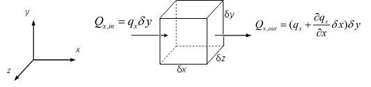
Figure 3: Conservation of flow in a control volume in Cartesian coordinate

The net flow in \(x\) axis is:

(13)\[Q_{x,net} = Q_{x,out}-Q_{x,in}=\frac{\partial q_x}{\partial x}\delta x \delta y\]

and in \(y\) axis is:

(14)\[Q_\mathrm{y,net} = Q_\mathrm{y,out}-Q_{y,in}=\frac{\partial q_y}{\partial y}\delta y \delta y\]

The constant pressure along \(z\) axis make the net flow rate in this direction dominated by the fluid loss rate through the fracture surface:

(15)\[Q_L = q_L \delta x \delta y\]

and \(q_L\) is the fluid loss rate per unit fracture surface that can be expressed by Carter’s equation:

(16)\[q_L = \frac{2C_L}{\sqrt{t-t_0(x,y)}}\]

where: \(C_L\) is the Carter’s leakoff coefficient and \(t_0(x,y)\) represents the time at which the point of fracture surface gets exposed to the fluid.

Since the rate of the fracture volume increase (storage effect) is \(\frac{\partial V}{\partial t}=\frac{\partial w}{\partial t}\delta x \delta y\), the flow conservation leads to:

(17)\[Q_\mathrm{x,net}+Q_{y,net}+Q_L+\frac{\partial V}{\partial t}=0\]

Substitution Eqn (13) through Eqn (15) into Eqn (17) and cancel the \(\delta x \delta y\) term:

(18)\[\frac{\partial q_x}{\partial x} + \frac{\partial q_y}{\partial y} + \frac{2C_L}{\sqrt{t-t_0(x,y)}} + \frac{\partial w}{\partial t}=0\]

Eqn (18) is called the fluid flow continuity equation in the Cartesian coordinate. Substitution of Eqn (12) into Eqn (18) yields the Reynolds equation (Eqn (19)) that governs the fluid pressure distribution in the fracture in Cartesian coordinate:

(19)\[\frac{1}{12\mu} \frac{\partial}{\partial x}( w^3\frac{\partial p}{\partial x} ) + \frac{1}{12\mu} \frac{\partial}{\partial y}( w^3\frac{\partial p}{\partial y} ) = \frac{2C_L}{\sqrt{t-t_0(x,y)}} + \frac{\partial w}{\partial t}\]

Cylindrical coordinate¶

In the Cylindrical coordinate the lubrication theory yields:

\[\begin{split}\left\{ \begin{align} & \frac{\partial p}{\partial r} = \mu\frac{\partial^2 u_r}{\partial z^2} \\ & \frac{1}{r} \frac{\partial p}{\partial \theta} = \mu\frac{\partial^2 u_\theta}{\partial z^2} \\ \end{align} \right.\end{split}\]

Integration of the above equations with respect to \(z\) with the non-slip boundary conditions (5th assumption of the lubrication theory) for fracture width \(w(r,\theta,t)\) (zero velocity at \(\pm \frac{w}{2}\))gives:

(20)\[\begin{split}\left\{ \begin{align} & u_r = -\frac{1}{2\mu}[\frac{w^2}{4}-z^2]\frac{\partial p}{\partial r} \\ & u_\theta = -\frac{1}{2\mu r}[\frac{w^2}{4}-z^2]\frac{\partial p}{\partial \theta} \\ \end{align} \right.\end{split}\]

The volumetric flow rate per unit fracture length is then:

(21)\[\begin{split}\left\{ \begin{align} & q_r = \int_{-\frac{w}{2}}^{\frac{w}{2}}u_rdz = -\frac{w^3}{12\mu}\frac{\partial p}{\partial r} \\ & q_\theta = \int_{-\frac{w}{2}}^{\frac{w}{2}}u_\theta dz = -\frac{w^3}{12\mu r}\frac{\partial p}{\partial \theta} \\ \end{align} \right.\end{split}\]

Consider a control volume marked in red as shown in Figure 4. The two vertical edges \(\delta r\) and two arc sides \(r \delta \theta\) and \((r+\delta r) \delta \theta\) are fixed side (only the width \(w\) in \(z\) direction changes with time):

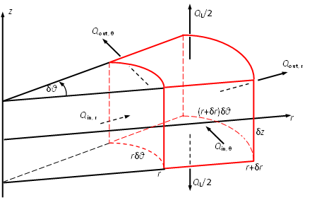
Figure 4: Conservation of flow in a control volume in Cylindrical coordinate

Similarly, the net flow in \(\theta\) direction is:

(22)\[Q_{\theta,net} = Q_{\theta,out}-Q_{\theta,in} = (q_\theta + \frac{\partial q_\theta}{\partial \theta}\delta \theta)\delta r - q_\theta \delta r = \frac{\partial q_\theta}{\partial \theta}\delta \theta\delta r\]

The net flow in \(r\) direction is:

(23)\[\begin{split}\begin{equation} \begin{split} Q_\mathrm{r,net} &= Q_\mathrm{r,out}-Q_{r,in} \\ &= (q_r + \frac{\partial q_r}{\partial r}\delta r)(r+ \delta r)\delta \theta - q_r r \delta \theta \\ &= q_r \delta r \delta \theta + \frac{\partial q_r}{\partial r}r \delta r \delta \theta \end{split} \end{equation}\end{split}\]

And the net flow in \(z\) direction is dominated by the fluid leakoff rate through the fracture surface:

(24)\[Q_L = q_Lr \delta\theta \delta r\]

Since the rate of the fracture volume increase (storage effect) is \(\frac{\partial V}{\partial t} = \frac{\partial w}{\partial t}r \delta r \delta \theta\), the flow conservation leads to:

(25)\[Q_\mathrm{r,net}+Q_{\theta,net}+Q_L+\frac{\partial V}{\partial t}=0\]

Substitution Eqn (22) through Eqn (24) into Eqn (25) and cancel the \(\delta r \delta \theta\) term:

(26)\[\frac{1}{r}\frac{\partial rq_r}{\partial r} + \frac{1}{r}\frac{\partial q_\theta}{\partial \theta} + \frac{2C_L}{\sqrt{t-t_0(x,y)}} + \frac{\partial w}{\partial t}=0\]

Eqn (26) is called the fluid flow continuity equation in the Cartesian coordinate. Substitution of Eqn (21) into Eqn (26) yields the Reynolds equation (Eqn (27)) that governs the fluid pressure distribution in the fracture in Cylindrical coordinate:

(27)\[\frac{1}{12\mu r} \frac{\partial}{\partial r}( rw^3\frac{\partial p}{\partial r} ) + \frac{1}{12\mu r^2} \frac{\partial}{\partial \theta}( w^3\frac{\partial p}{\partial \theta} ) = \frac{2C_L}{\sqrt{t-t_0(x,y)}} + \frac{\partial w}{\partial t}\]

• Special case: Axisymmetric flow without tangential velocity

  For the axisymmetric flow (\(\frac{\partial}{\partial \theta}=0\)) without the tangential velocity (\(u_\theta=0\)), the Reynolds equation Eqn (27) is reduced to:

  (28)\[\frac{1}{12\mu r} \frac{\partial}{\partial r}( rw^3\frac{\partial p}{\partial r} ) = \frac{2C_L}{\sqrt{t-t_0(x,y)}} + \frac{\partial w}{\partial t}\]

Note

The Reynolds equation is the result of the application of the lubrication theory on hydraulic fracturing.

Governing equation of KGD radial model¶

The Kristianovich-Geertsma-de Klerk (KGD) radial model is a classic 2D hydraulic fracturing model, named in honor of three researchers who greatly contributed to it. [1] The following assumptions are used in the model: [2]

1. The formation is an infinite, homogeneous, isotropic, linear elastic medium characterized by Young’s modulus \(E\) , Poisson’s ratio \(\nu\) and toughness \(K_{Ic}\).

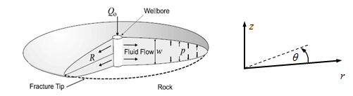
Figure 5: Schematic view of the KGD radial model geometries

2. The fracture is assumed to be radially symmetric and generated from a point-source at its center. The periphery of the fracture is circular (penny-shaped), as shown in Figure 5. [3]
3. The Newtonian fracturing fluid with viscosity \(\mu\) is injected with a constant volumetric flow rate \(Q_0\), and its flow is laminar. Gravitational effects are not taken into account.

The fracture width (measurable in millimeter) is significantly smaller than the radius (tens to hundreds of meters) so that the lubrication theory in the cylindrical coordinate is convenient for the KGD radial model. Besides the fluid is unidirectional (\(r\) direction) and the geometry is radially axisymmetric, thus the Reynolds equation Eqn (28) is directly applicable for this model. When the fluid leakoff is excluded, Eqn (28) is reduced to:

where: \(\mu'=12\mu\)

Governing equation of PKN model (Nordgren equation)¶

The Perkins-Kern-Nordgren (PKN) model is another well-known 2D classic hydraulic fracturing model with a long fracturing length (hundreds of meters in length, x-axis as shown in Figure 6), limited but constant height (tens of meters in y-axis) and small width (measurable in millimeters in z-axis) propagated in an infinite homogeneous isotropic linear elastic formation characterized by Young’s modulus \(E\), Poisson’s ratio \(\nu\) and toughness \(K_{Ic}\). [4]

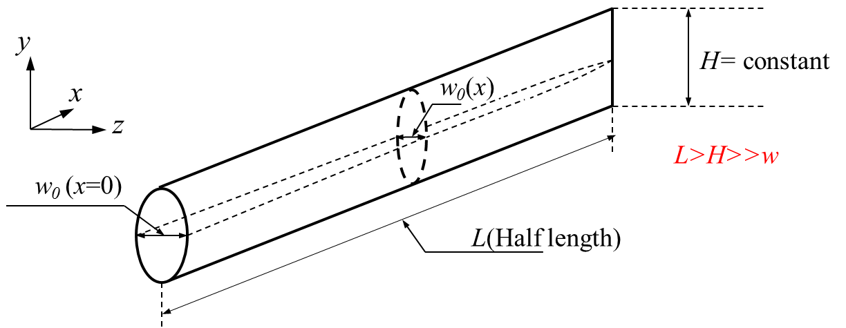
Figure 6: Schematic view of the PKN model (one-wing)

Because the fracture length is large compared to the other two ones, the approximate plane strain condition can be assumed in every plane orthogonal to the length (x-axis) [5], which means the net pressure on different vertical planes are not the same as for the exact plane strain condition, but the net pressure is independent of y-axis and the fracture width is calculated from the plane strain solution with this constant pressure on a single vertical plane, making the cross section elliptical [6]:

where: \(w\) and \(p\) are the fracture width and fluid net pressure respectively in a vertical plane and the plane strain Young’s modulus \(E'\) is defined as:

The fracture width at the center of a vertical plane is then given by [6]:

Typically, when the fracture total length (\(2L\)) is more than three times of the height, the error from the plane strain assumption is negligible [7].

Besides the approximate plane strain condition, the PKN model is based on another assumption that the fluid flow inside the fracture is incompressible Newtonian laminar unidirectional (\(x\) axis in Figure 6) flow characterized by viscosity \(\mu\) and the gravity effect is not taken into account.

The known slit-like elliptical cross-section (\(z \ll x,y\)) profile due to the plane strain assumption needs further treatment compared to the previous analysis in the Cartesian coordinate. Thus, the analysis here starts from the original NS equation Eqn (1) in Cartesian coordinate for a fluid flow passing through a long straight elliptic cross-section pipe as shown in Figure 7.

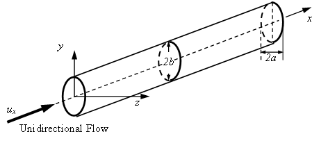
Figure 7: A unidirectional flow in a long straight elliptic cross-section pipe

The PKN assumptions associated with the lubrication theory (\(z \ll x, y\)) yield:

• \(p\) is independent of \(y\) and \(z\) due to plane-strain condition;
• \(u_y=u_z=0\) due to unidirectional flow;
• \(\rho=0\) because no gravity effect.

and reduce the original NS equation Eqn (1) to:

Because the fracture length in \(x\) direction in Figure 7 is much larger than the others, the lubrication theory can be applied with \(\frac{\partial u_x}{\partial x}=0\) to reduce Eqn (33) to:

The elliptic cross-section shape corresponds to an ellipse with axes of width \(2a\) and height \(2b\):

The boundary of the ellipse is the locus of points (\(x,y\)) such that:

Note that:

By inspection Eqn (36) and Eqn (37), we can find out a solution to Eqn (34) with non-slip boundary conditions (\(u=0\) on the ellipse boundary):

Then the average fluid velocity \(\bar u_x\) passing through the elliptic cross-section of area \(\pi ab\) is:

The last second procedure of Eqn (39) is from the integral of an oven function, and the \(-1\) term in the integral actually leads to the \(1/4\) of the ellipse area (\(\pi ab/4\)), thus:

The details on how to get the integrals can be found from here.

Replace \(a\) and \(b\) in Eqn (40) with \(\frac{w_0}{2}\) and \(\frac{H}{2}\) defined in Figure 6:

Because the fracture width (millimeters) is significantly smaller than the height (tens of meters), \(\frac{w_0}{H}=0\) can be assumed and substituted into Eqn (41) to get:

Then the fluid flow per unit fracture height \(q_x\) is:

For an infinitesimal elliptic element with fixed side \(\delta x\) and \(\delta y\) as shown in Figure 8:

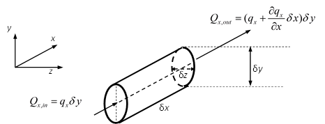
Figure 8: Conservation of flow in a elliptic control volume

The net flow in \(x\) axis is

There is no flow in \(y\) directions because of the unidirectional flow, and the net flow rate in \(z\) direction is dominated by the fluid leakoff rate through the fracture surface:

where:

• \(e\) is the eccentricity of the infinitesimal elliptic cross-section and \(e=\sqrt{1-(\frac{\delta z}{\delta y})^2} \rightarrow 1\) because the fracture width is significantly smaller than height;
• \(J\) represents the complete elliptic integral of the second kind so that \(\delta yJ(e)\) equals to half perimeter of the elliptic cross-section.

\(J\) is a function of a single argument. \(J(e)\) presents the value of \(J\) when the argument equals to the eccentricity, instead of \(J \times e\). Since \(e \rightarrow 1\), \(J(e)=J(1)=1\). Thus, Eqn (45) becomes:

And the rate of the fracture volume increase (storage effect) is \(\frac{\partial V}{\partial t}=\frac{\pi}{4}\frac{\partial w_0}{\partial t} \delta y \delta x\). The flow conservation leads to:

Substitute Eqn (44) and Eqn (46) into Eqn (47) to get:

Substitute Eqn (32) and Eqn (43) into Eqn (48):

Notice that: \(w_0^3\frac{\partial}{\partial w_0^3}=\frac{1}{4} \frac{\partial w_0^4}{\partial x}\), the governing equation of PKN model is then obtained after some arrangement: