Pumping Schedule
This panel is where the pumping schedule is specified. Central to this panel is the table where the user inputs data to set up the pumping schedule. Below that is a plot of the pumping schedule that is updated as the schedule is modified.
Schedule Type
Prior to inputting any specific data to construct the pumping schedule, the type of this schedule should be defined by choosing one of the two choices (Figure 1).
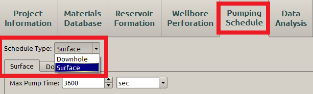
Figure 1: Two types of pumping schedule
The Downhole type (Figure 2) characterizes the pumping parameters right at the downhole (Figure 3); while the Surface type (Figure 4) characterizes the pumping parameters at the surface. Usually, the input data correspond to the surface pumping because it is easier to be controlled in the real situation.
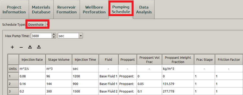
Figure 2: Downhole pumping schedule
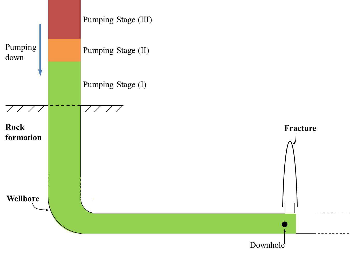
Figure 3: A wellbore during a pumping
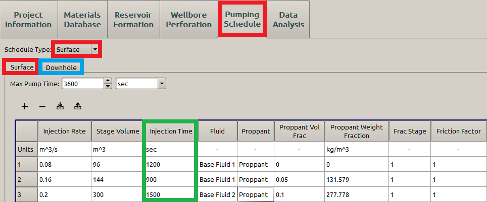
Figure 4: Surface pumping schedule
When the Downhole type is chosen, the computation is simpler because users can directly model the pumping at the downhole by changing parameters. However, when the Surface type is chose, it gets more complicated to model the whole pumping schedule. Because when users specify the surface pumping schedule directly, the downhole pumping (the blue box in Figure 4) needs changing accordingly with the change at the surface. Thus, the downhole pumping schedule under the Surface type is read only (Figure 5). It is interpreted from the surface one instead of being specified by users.
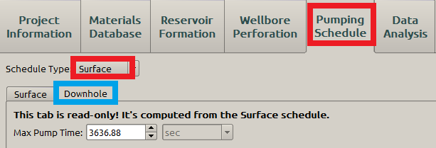
Figure 5: Surface pumping schedule
Interpretation of the downhole pumping schedule from the surface one
When the pumping schedule is set up in the Surface type as illustrated in Figure 4, there are three surface pumping stages:
- Pumping Stage \(\mathrm{I}\): Fluid (1) consisting of Base Fluid 1 and no proppant (green in Figure 3);
- Pumping Stage \(\mathrm{II}\): Fluid (2) consisting of Base Fluid 1 and low proppant concentration (orange in Figure 3);
- Pumping Stage \(\mathrm{III}\): Fluid (3) consisting of Base Fluid 2 and higher proppant concentration (red in Figure 3);
The pumping stage defined in FrackOptima is a group of parameters including pumping rate, fluid, proppant, proppant volume fraction, frac stage and friction factor. If one of these parameters change, the pumping stage differs from the original one. For a specific pumping schedule table, each line corresponds to an individual pumping schedule. For example, there are three pumping stages for the surface pumping schedule in Figure 4.
Once a surface pumping schedule is defined (Figure 4), the downhole one can be interpreted as illustrated in Figure 6.
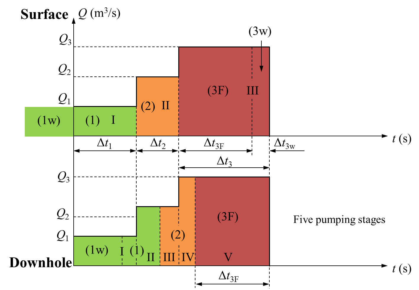
Figure 6: Downhole pumping schedule interpretation
In Figure 6,
- \(\mathrm{(1)}\), \(\mathrm{(2)}\) and \(\mathrm{(3)}\) represent Fluid (1), Fluid (2) and Fluid (3). These three fluids are marked in green, orange and red, respectively. Thus, the same color indicates the same fluid;
- \(\mathrm{(3F)}\) is the part of Fluid (3) that flows in the fractures; while \(\mathrm{(3w)}\) is the part of Fluid (3) that stays in the wellbore.
- \(\triangle t_1\) to \(\triangle t_3\) are injection time of the three stages (green box in Figure 4).
FrackOptima treats the fluid in a wellbore prior to a pumping schedule as in the same pumping stage as the first stage of that schedule (the green box labeled by \(\mathrm{(1w)}\) and to the left of the vertical axis of the surface pumping schedule in Figure 6). Then, that fluid is defined to be pumped through the downhole as the same fluid at the same injection rate as the one in the first pumping stage in FrackOptima.
The downhole pumping schedule (the lower part in Figure 6) is supposed to be in the same form of the surface one (same injection rates \(\mathrm{Q}\) and times \(\triangle t\)) to maintain the synchronization of the two pumping schedules. As a result, there must be a pumping shift in the downhole schedule compared to the surface one. For example, all the Fluid (1) is pumped at the injection rate \(Q_1\) on the surface in the surface pumping schedule. However, only part of the Fluid (1) can be pumped through the downhole at \(Q_1\), because it takes some time to pump Fluid \(\mathrm{(1w)}\), which stays in the wellbore before the surface pumping starts, through the downhole so that the new Fluid (1) can reach the downhole. After all the Fluid \(\mathrm{(1w)}\) passes the downhole, the new Fluid (1) begins to pass downhole at \(Q_1\). When the pumping time reaches \(\triangle t_1\), the part of Fluid (1) that has not passed downhole yet will be pumped through downhole at the different injection rate \(Q_2\). As defined above, with a change in the injection rate, the pumping stage changes. Therefore, the new stage (Stage \(\mathrm{II}\)) starts from \(\triangle t_1\) even the fluid being pumped remains the same. In Figure 6, this procedure is illustrated as the Fluid (1) divided into Stage \(\mathrm{I}\) and \(\mathrm{II}\) in the downhole pumping schedule. In the same manner, Fluid (2) is divided into Stage \(\mathrm{III}\) and \(\mathrm{IV}\); while only Fluid \(\mathrm{(3F)}\) is pumped through downhole. Because when the time reaches the end time, both pumping stops, leading to Fluid \(\mathrm{(3w)}\) remaining in the wellbore. Therefore, the three pumping stages of the surface pumping schedule is interpreted to five stages of the downhole one.
Other parameters
Max Pumping Time
The Max Pumping Time specifies the stop time \(\mathrm{t_{stop}}\) for simulation. If the largest injection time \(\mathrm{t_{i,max}}\) defined in the pumping schedule matrix is larger than the max pumping time, the simulation stops when the time reaches \(\mathrm{t_{stop}}\) (see the red bar in Figure 7). When \(\mathrm{t_{i,max}<t_{stop}}\), the simulation resumes with treating the injection rate as \(0\).
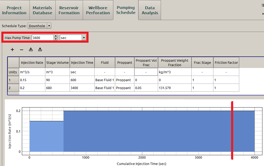
Figure 7: Pumping schedule
For example, the simulation stops when the time reaches the Max Pumping Time \(\mathrm{3600 s}\), although the scheduled pumping lasts for \(\mathrm{4000 s}\) in Figure 7. This is useful if users only want to simulate part of your pumping schedule.
Pump Proppant
This specifies which proppant defined in Proppant subpanel is used in the fracking fluid. Currently, only one proppant can be used in a single pumping stage (one row of the pumping schedule table).
Pumping Schedule Table
This table contains some sets of columns that depend on one another. Each group will be explained here. Otherwise, this table functions just like any other table. For the \(i\textrm{th}\) row of the table:
Injection Rate: denoted by \(\mathrm{Q_i}\), is the volumetric injection rate. The injection rate for an unconventional reservoir usually reaches up to \(\mathrm{100 bbl/min}\), or \(\mathrm{0.26 m}^3/\mathrm{s}\);
Injection Time: denoted by \(\mathrm{t_i}\) , specifies the duration of each pumping row. For example, there are two rows in the pumping schedule in Figure 7. The first one lasts \(600\) seconds and the second one lasts \(3400\) seconds, for a total of \(4000\) seconds.
Stage Volume: denoted by \(\mathrm{V_i}\), is the total volume pumped into the rock formation in the \(i\textrm{th}\) row defined by the equation:
(1)\[V_i = Q_i(t_\mathrm{i} - t_\mathrm{i-1})\]Proppant Volume Fraction and Proppant Weight Fraction: denoted by \(\phi\) and \(\omega\), respectively, are two different measures of the proppant concentration in the slurry. \(\phi\) and \(\omega\) can be related using the proppant density \(\rho\):
(2)\[\phi = \frac{\omega}{\rho + \omega}\]
The Proppant Weight Fraction here represents the mass of the proppant in a unit volume of clean fluid:
(3)\[\omega = \frac{m_p}{V_f}\]
where:
- \(m_p\) : the mass of proppant
- \(V_f\) : the volume of clean fluid
Pumping Schedule Plot
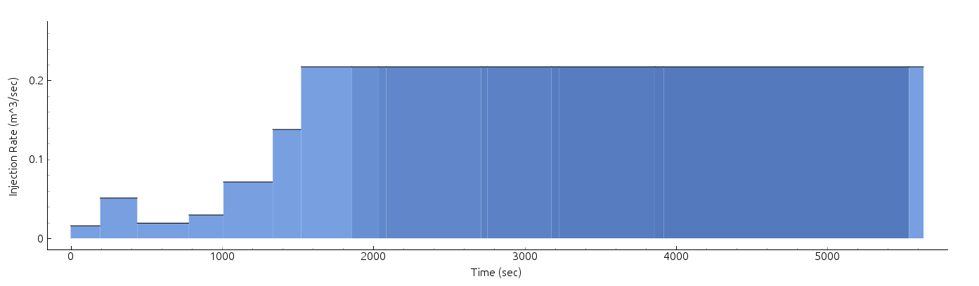
Figure 8: A schematic pumping schedule including various proppant concentrations and injection times
The pumping schedule plot gives a visual representation of the pumping schedule. More particularly, it is a plot of the injection rate versus injection time. The color of each part of the plot is based off of the proppant fraction, where a lighter color means a lower concentration and a darker color means a higher concentration. This is useful to help the user visualize relative magnitudes of injection times and proppant concentrations (see Figure 8 for example).
Just like many other plots, right click the plot to bring up a context menu. The context menu items are explained in the Context Menu section. However, changing plot units is done with the pumping schedule table, not the context menu.
See also
- Plot Controls
- For more information on how to control the plot.