Reservoir Stress
Stress Table
Introduction
The input in-situ stress in Reservoir Formation Stress subpanel (Figure 1) assumes uniform stress distribution on defined horizontal planes. For example, the two horizontal normal stresses are \(\textrm{30 MPa}\) and \(\textrm{33 MPa}\) throughout the plane at Depth \(\textrm{-800 m}\) in Figure 1. However, Reservoir Stress panel inputs a more complex stress status of the reservoir for the simulation in the Reservoir Stress subpanel under Wellbore Perforation panel, which can specify shear stresses (e.g. \(S_{xy}\) ) and stresses of \(\textrm{z}\) (vertical) component on different points (East and North) at the same Depth, as shown in Figure 2.
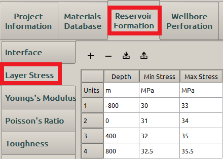
Figure 1: The Layer Stress subpanel of the Reservoir Formation panel
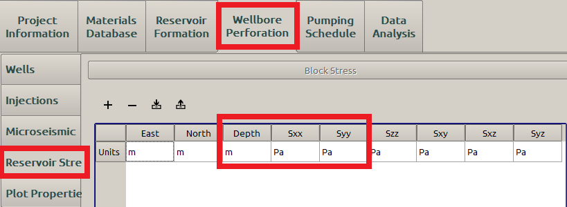
Figure 2: The Reservoir Stress subpanel of the Wellbore Perforation panel
The input stress table here (Figure 2) will be the same as the one in Reservoir Formation Stress subpanel (Figure 1), if only Depth, Sxx and Syy (the horizontal plane position and two horizontal normal stresses) are considered.
Import the stress
Here is an example to import the stress from an external file. The details of importing a file can be found here, thus the example here is a relative brief one. We first click the Import button (blue box in Fig 3)on the Reservoir Stress subpanel,
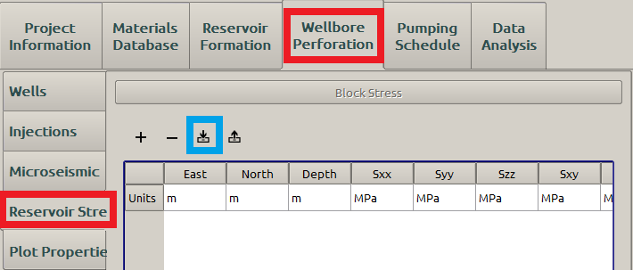
Figure 3: The import button
and then click the New button on the pop-up window (blue box in Figure 4) to set up a new fod file, and then click the load button (green box in Figure 4) to load data from a tabular file, which is a csv file here.
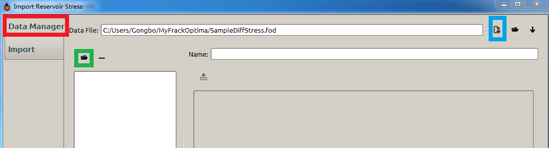
Figure 4: Stress import-Step 1
After that, a user finds the csv file called “SampleReservoirStress” by clicking the Browse button (blue box in Figure 5) on the following Select Tabular File pop-up window, and then load it by clicking OK (green box in Figure 5). Because there is only one sheet in the imported file so that the Excel Sheet Name option is grey (inactivated).
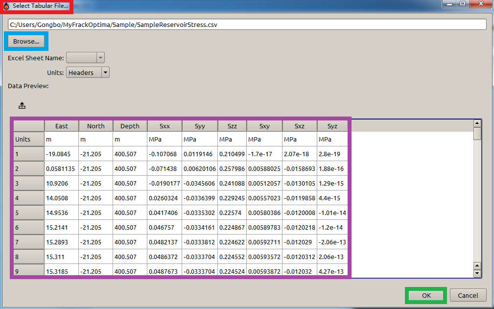
Figure 5: Stress import-Step 2
Then a preview of the imported data is available as shown in Figure 6.
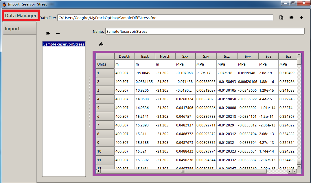
Figure 6: Stress import-Step 3
Then, the user goes to Import subpanel (red box in Figure 7), and click the Accept (blue box in Figure 7) to complete the import.
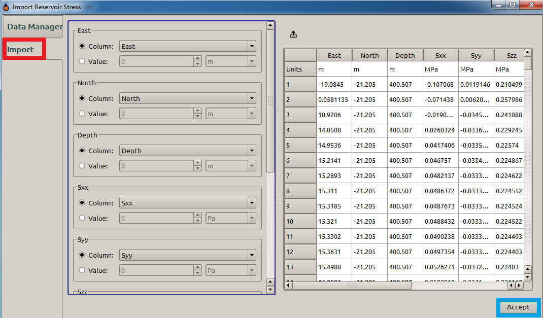
Figure 7: Stress import-Step 4
After clicking the Accept button in Figure 7, the user completes the stress data input, which is shown in the purple box in Figure 8.
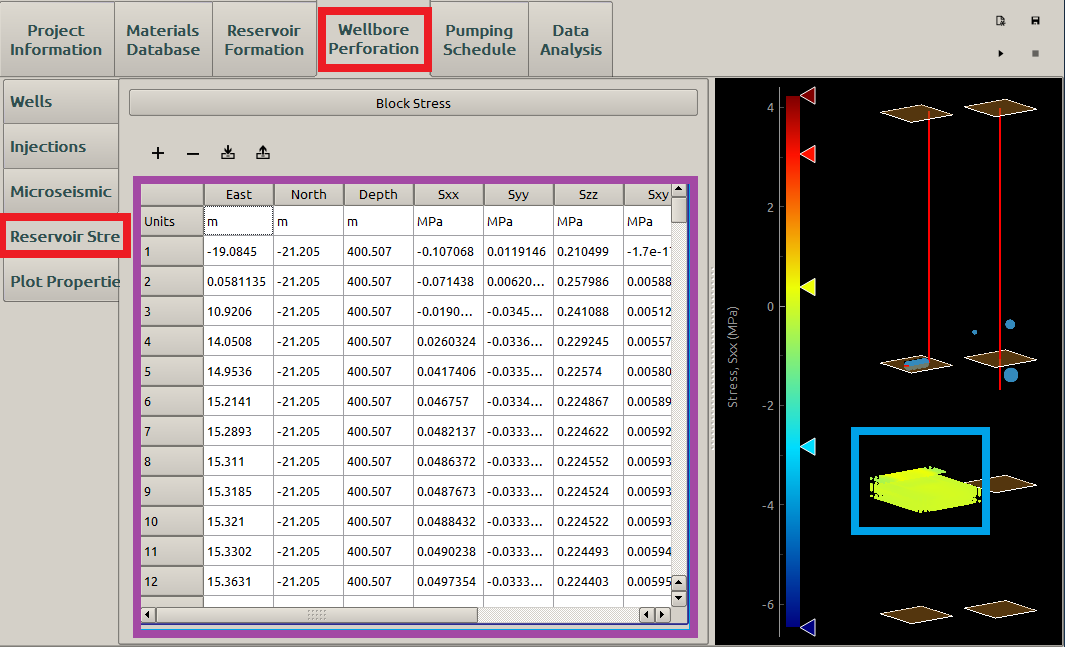
Figure 8: Stress import-Step 5 (complete)
In the plotting of Figure 8, the golden parts in the blue box represents the plotting of one component of the imported Reservoir Stress. As a default, the plotted component is \(S_{xx}\).
The values of these data are the difference between the stresses defined in Reservoir Formation (see Figure 1 for example), instead of the absolute stress value (the stresses defined in Reservoir Formation are the absolute stresses). The stress Sxx and Syy here are defined in East and North directions (see Figure 9), respectively. Then the two stresses can be decomposed to the \(\sigma_\textrm{h,min}\) and \(\sigma_\textrm{h,max}\) directions to obtain two new horizontal \(\sigma_\textrm{h,min}\) and \(\sigma_\textrm{h,max}\).
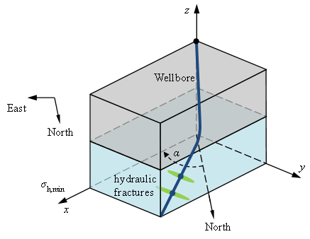
Figure 9: The minimum horizontal stress azimuth
Reservoir Stress in Plot Properties
The Plot Properties of the Wellbore Perforation provides a 3D visualization of the Reservoir Stress chosen in the Component option (Figure 10). In Figure 10, \(S_{yy}\) is chosen instead of \(S_{xx}\) in Figure 8.
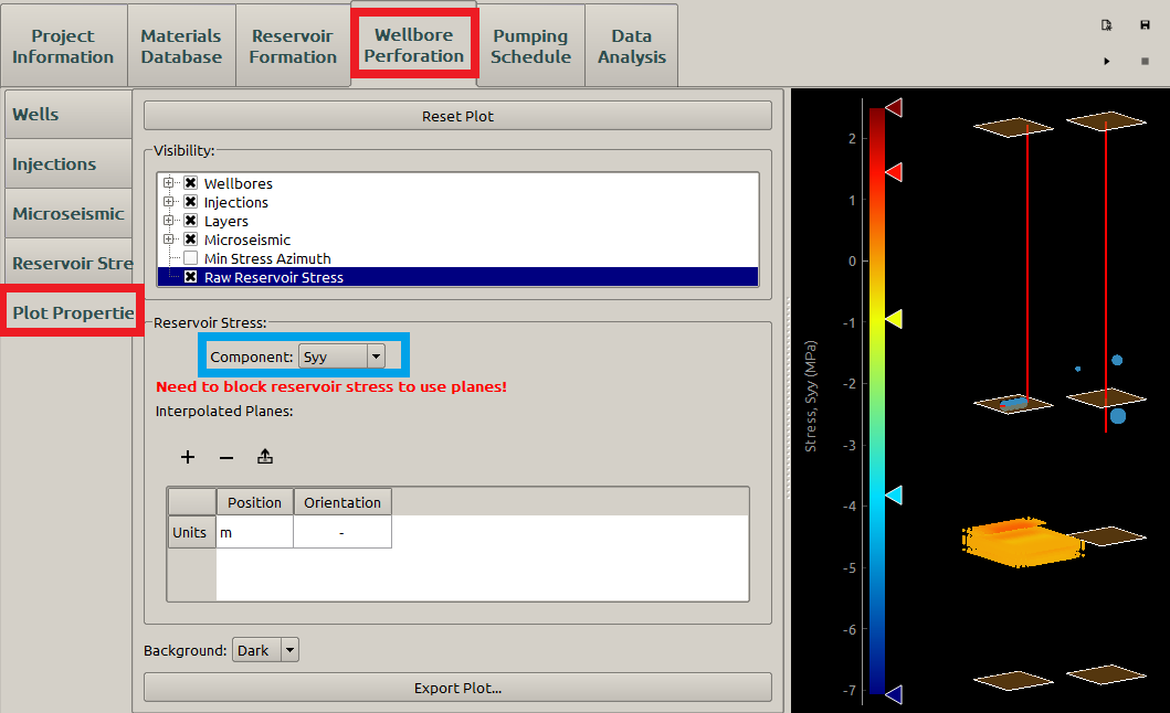
Figure 10: Stress plot
A user can insert an plane and examine the stress distribution on it. Before doing so, an interpolation needs carrying out to reduce the computation with a click on the Block Stress button (Figure 11)..
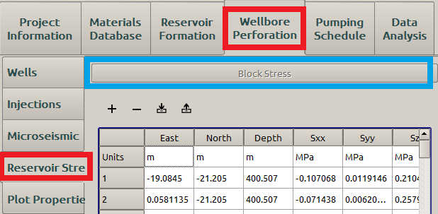
Figure 11: Stress interpolation
The discrete stress are then included in a grid cell with the size defined in the Reservoir Formation - Interface subpanel (Figure 12).
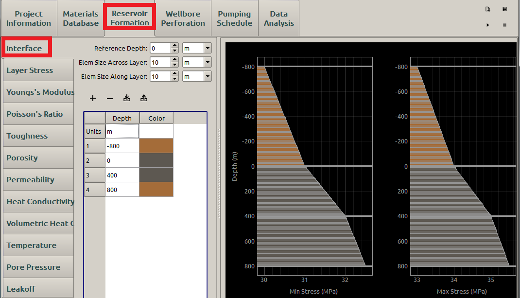
Figure 12: Interface inputs for reservoir formation
The cell has length and width as the Element Size Along Layer and height as the Element Size Across Layer. In this example, a cell is a \(\textrm{10 m}\)-length cubic. Inside each grid cell, an linear average interpolation is implemented for all the discrete stress points in it.
Then the user can insert planes defined by its orientation and position to examine the stress distribution on it (Figure 13).
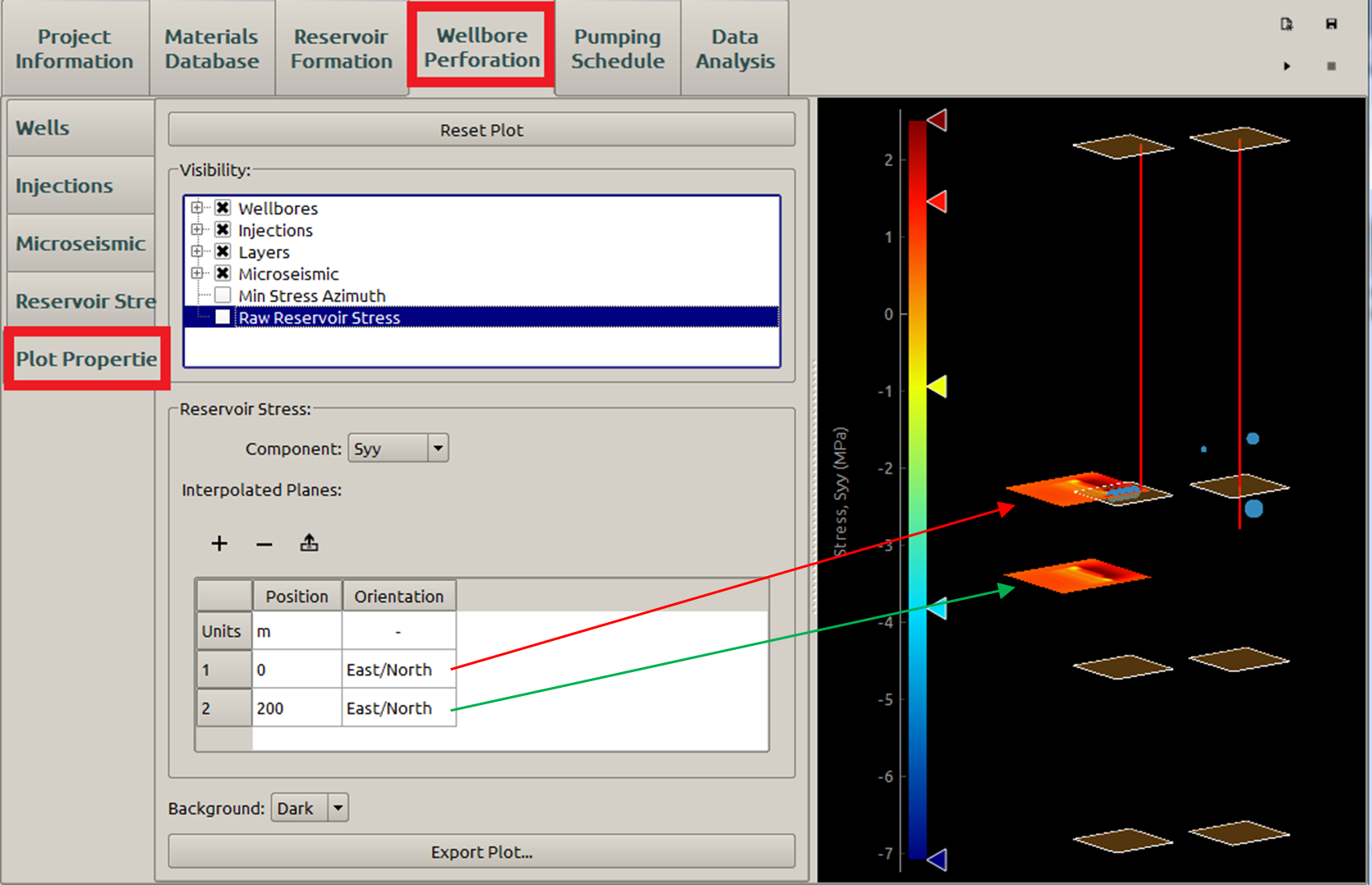
Figure 13: Stress on planes
Please notice that the Reservoir Stress plotting is unchecked in Figure 13.