Preliminary Mathematics
Bessel functions
Fundamental of Bessel functions
Bessel functions
The Bessel functions are the solution to the linear homogeneous second-order ODE, also known as Bessel equation, in the form for \(\alpha \in \mathbb{C}\):
where: \(\mathbb{C}\) represents the complex number set.
Then, two linearly independent particular solutions \(y_1(x)\) and \(y_2(x)\) have to be found to construct a general solution \(c_1y_1(x)+c_2y_2(x)\) with \(c_1,\ c_2\) both arbitrary constants.
One particular solution \(y(x)\) is given as:
Conventionally, the first particular solution \(y(x)\) is denoted by \(J_{\alpha}(x)\) with the full name: \(the \ \alpha th \ order \ Bessel \ function \ of \ the \ first \ kind\).
where: the function \(\Gamma(t)\) is the gamma function defined for the complex number \(t\) with positive real part as:
Integration by parts on Eqn (4) yields:
If \(t\) is a positive integer(\(t\in \mathbb{N}\)), \(\Gamma(t)\) can be defined as the factorial:
For non-integer \(\alpha\), the two functions \(J_{\alpha}(x)\) and \(J_{-\alpha}(x)\) are linearly independent, thus they are the two linearly particular independent solutions of the Bessel equation defined in Eqn (1).
Once \(\alpha\) is non-negative integer (\(\alpha = n \in \mathbb{N^0}\)), \(J_{\alpha}(x)\) and \(J_{-\alpha}(x)\) are no longer linearly independent. A second linearly independent particular solution denoted by \(Y_{\alpha}(x)\), called \(the \ \alpha th \ order \ Bessel \ function \ of \ the \ second \ kind\) is obtained as:
where:
- \(\varphi (t)=\frac{\Gamma'(t)}{\Gamma(t)}\), and \(\Gamma'(t)=\frac{d \Gamma}{dt}\)
- \(\mathbb{N^0}\) represents the non-negative integer set (\(n = 0,1,2......\)).
Sometimes the Bessel equation is given in the form for constant \(\omega \in \mathbb{R}\):
Then the solutions are given as \(J_{\alpha}(\omega x)\) and \(Y_{\alpha}(\omega x)\).
Particularly, for the Bessel function of order zero in the form:
Then the solutions are given as \(J_0(\omega x)\) and \(Y_0(\omega x)\).
\(\mathbb{R}\) represents the real number set.
Modified Bessel functions
An important special case for the Bessel equation is for argument \(x\) purely imaginary, i.e. \(x\) is replaced by \(xi\) so that Eqn (1) becomes to:
Eqn (8) is called the modified Bessel equation and the solutions are:
where:
- \(I_{\alpha}(x)\) is the \(\alpha th\) order modified Bessel function of the first kind
- \(K_{\alpha}(x)\) is the \(\alpha th\) order modified Bessel function of the second kind
Similarly, for the second-order ODE of the form:
Then the solutions are given as \(I_{\alpha}(\omega x)\) and \(K_{\alpha}(\omega x)\).
And for the modified Bessel equation of zero order as Eqn (11), the solution is \(I_0(\omega x)\) and \(K_0(\omega x)\).
Preliminaries of the application of the Bessel functions on the wellbore heat transfer problems
Consider an infinite axisymmetric cylinder without heat generation inside but with radial heat flow only, the governing equation (see here for details) :
will be reduced to Eqn (12):
With the boundary condition (BC) and initial conditions (IC):
The function \(f(r)\) is a known function or \(r\) only.
The separation of variables method looks for simple-type solutions to PDE Eqn (12) of the form:
where: \(u\) is a function of \(r\) only and \(v\) is a function of \(t\) only.
Substitution of Eqn (14) into Eqn (12):
where: \(\dot v = \frac{dv}{dt}, and \ \ u'=\frac{du}{dr}\) .
Rearranging Eqn (15) leads to:
Because \(r\) and \(t\) are independent of each other, then each side of Eqn (16) must equal to a fixed constant \(\beta\):
The left side of Eqn (17) yields:
The solution to Eqn (18) is:
\(C_1\) is an arbitrary constant. Observation on Eqn (19) indicates that \(\beta\) has to be negative otherwise \(v\) tends to be infinity as \(t \rightarrow \infty\). Thus, \(\beta=-\mu^2\) (\(\mu \in \mathbb{R}\)):
Consequently, the whole solution is of the form:
The right side of Eqn (17) yields:
which is the Bessel function of order zero (with \(x,y\) replaced by \(r,u\) in Eqn (7)).
Because the Bessel function of the second kind (Eqn (5)) is infinite at \(r=0\), the particular solution to Eqn (22) is of the form in the Bessel function of the first kind:
Consequently, the solution to the PDE Eqn (12) is:
To satisfy the boundary condition Eqn (13), \(\mu\) must be a root of the equation:
It is known that Eqn (25) has no complex roots or repeated roots and that it has an infinite number of real positive roots: \(\mu_1, \mu_2, ...\). Also, to each positive root \(\mu\), there corresponds a negative root \(-\mu\).
In addition, the initial condition \(f(r)\) in Eqn (13) is known to be expanded in the “Fourier-Bessel” series as follows and can be integrated term by term:
Therefore, the solution to Eqn (12) can be written as:
If the boundary condition is the radiation at the surface to the medium at zero temperature:
where:
- \(\mathbf{n}\) is the outward normal direction to the surface;
- \(k\) is the heat conductivity of the medium;
- \(H\) is the constant proportionality of the heat flow and temperature difference.
Then the solution is still in the form as Eqn (27), while \(\mu\) is the root of the equation:
Then, the last task is evaluating the coefficients \(A_m\) in Eqn (27), which can be obtained from the two tables below listing the values of the integrals, with \(h=H/k\) and \(n \in \mathbb{N^0}\):
| \(\mu, \lambda\) are two different positive roots of | Value of \(\int_0^{r_w}rJ_n(\mu r)J_n(\lambda r)dr\) |
|---|---|
| \(J_n(\mu r_w)=0\) | \(0\) |
| \(J_n'(\mu r_w)=0\) | \(0\) |
| \(\mu J_n'(\mu r_w) + hJ_n(\mu r_w)=0\) | \(0\) |
And
| \(\mu\) is a positive roots of | Value of \(\int_0^{r_w}r[J_n(\mu r)]^2dr\) |
|---|---|
| \(J_n(\mu r_w)=0\) | \(\frac{r_w^2}{2}[J_n'(\mu r_w)]^2\) |
| \(J_n'(\mu r_w)=0\) | \(\frac{r_w^2}{2} (1-\frac{n^2}{\mu^2 r_w^2}) [J_n(\mu r_w)]^2\) |
| \(\mu J_n'(\mu r_w) + hJ_n(\mu r_w)=0\) | \(\frac{1}{2\mu^2} (r_w^2h^2+ \mu^2r_w^2-n^2) [J_n(\mu r_w)]^2\) |
In addition, the following formulae on Bessel function are also important for the application:
and for any \(\mu\), and \(n >-1\):
where: \(\mu\) must be a root of the equation \(J_0(\mu r_w)=0\):
and for \(n = 0\) and \(x \in \mathbb{R}\)
Note
For details of the Bessel functions, user can check Ref.1 [1] .
Application on the heat transfer problem for an infinite circular cylinder
This part mainly discuss how to apply Bessel functions on the examples of heat transfer problems for an infinite circular cylinder with three basic different boundary and initial conditions, from which solutions with more complicated conditions can be derived.
The infinite cylinder, prescribed surface temperature \(\varphi(t)\) at \(r=r_w\) and the initial temperature \(f(r)\)
When \(\varphi(t)=0\), it is the problem to initiate the preliminaries of the Bessel function application (see here), with \(f(r)\) expanded into Bessel-Fourier series:
where: \(\mu_m\) are positive roots of the equation and \(m \in \mathbb{N^0}\)
Multiplying both sides of Eqn (33) by \(rJ_0(\mu_m r)\), integrating from \(0\) to \(r_w\), and using the integral results of the two tables and the equation , namely (with \(\alpha=0\)):
The coefficients \(A_m\) is obtained:
Then the solution (the temperature) is:
If \(f(r)=T_0\) constant, the solution can be simplified by using the equation:
If \(f(r)=0\) and \(\varphi(t)=T_0\) for \(t>0\), the solution is obtained by subtracting Eqn (37) from \(T_0\):
It would be more convenient to use a dimensionless time \(t_D\) and a new variable \(\gamma_m\) defined as follows in the numerical analysis:
Consequently, Eqn (38) becomes:
Note
- This is how the dimensionless time \(t_D\) in Ramey solution is introduced;
- The series of Eqn (40) converges quite rapidly except for small \(t_D\), as a consequence, alternative solutions suitable in this case is needed with the Laplace transformation.
If \(f(r)=0\) and \(\varphi(t)\) is given, the Duhamel’s theorem applies on Eqn (38). First, take \(T_0=1\):
Substitution Eqn (41) into the equation :
The infinite cylinder, radiation at the surface \(r=r_w\) and the initial temperature \(f(r)\)
The \(f(r)\) is also expanded into Bessel-Fourier series:
where: \(\mu_m\) are positive roots of the equation (see here):
From the similar procedure as previously and the results in the two tables :
We have:
The infinite cylinder, constant flux \(F_0\) at the surface \(r=r_w\) and the initial temperature zero
The solution can be obtained in a similar manner:
Note
For the details of the application of the Bessel functions on heat transfer problems in an infinite circular cylinder, user can check Section 7 .1-7.8 in Ref.2 [2] .
Duhamel’s theorem
If the boundary condition (BC) is a given function of time \(t\), say \(\varphi(t)\), then the Duhamel’s theorem is needed to get the solution, which is presented as:
If \(v=F(x,y,z,\lambda, t)\) represents the temperature at point \((x,y,z)\) at time \(t\) in a solid in which the initial condition (IC) temperature is zero while its surface temperature is prescribed function \(\varphi=F(x,y,z,\lambda, t)\):
where: \(A(x,y,z)\) is a known function.
Then the solution of the problem in which the IC is zero and surface temperature is \(\varphi=F(x,y,z,t)\) is given by:
Proof
When the surface temperature is \(0\) from \(t=-\infty\) to \(t = 0\) and \(\varphi(x,y,z,\lambda)\) from \(t = 0\) to \(t = t\),we may say that the initial temperature is \(0\) and the surface temperature is \(\varphi(x,y,z,\lambda)\), so that the temperature \(v_0\) at the time \(t\) is given by:
Therefore, when the surface temperature is \(0\) from \(t=-\infty\) to \(t=\lambda\) and \(\varphi(x,y,z,\lambda)\) from \(t=\lambda\) to \(t=t\), we have the temperature \(v_1\):
Similarly, when the surface temperature is \(0\) from \(t=-\infty\) to \(t=\lambda+d\lambda\) and \(\varphi(x,y,z,\lambda)\) from \(t=\lambda+d\lambda\) to \(t=t\), we have the temperature \(v_2\):
Hence, when the surface temperature is \(0\) from \(t=-\infty\) to \(t=\lambda\); then \(\varphi(x,y,z,\lambda)\) from \(t=\lambda\) to \(t=\lambda+d\lambda\), and then \(0\) from \(t=\lambda+d\lambda\) to \(t=t\), we have the temperature \(v\):
The deduction of Eqn (49) to Eqn (52) can be illustrated in Figure 1
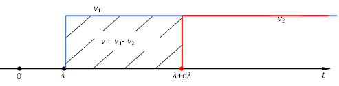
Figure 1: Illustration of the Duhamel’s theorem
Take \(d\lambda\) infinitesimal, \(v\) is ultimately:
In this way, by breaking up the interval \(t=0\) to \(t=t\) into these small intervals and then summing the results thus obtained, the solution to the problem can be found for the surface temperature \(\varphi(x,y,z,t)\) in the form:
Particularly, if \(v=F(x,y,z,t)\) represents the temperature at point \((x,y,z)\) at time \(t\) in a solid in which the initial temperature is \(0\) while its surface is kept at temperature unity, then the solution of the problem when the surface is kept at temperature \(\varphi(t)\) is given by:
This is the simpler case that \(F(x,y,z,\lambda,t)=F(x,y,z,t)\cdot \varphi(\lambda)\)
Note
For the details , user can check Section 1.14 in Ref.2 [2] .
Complex Analysis
As indicated in the Bessel function application, the solutions in terms of Bessel functions converges slowly when the dimensionless time \(t_D=\frac{\kappa t}{r_w^2}\) is small, which calls for alternative solutions based on Laplace transformation. The Laplace transformation transform many relationships and operations over the original function \(f(t)\) to a simpler ones over its image \(\bar{f}(s)\) in the integral form. Once \(\bar{f}(s)\) is obtained, it is usually necessary to get the original \(f(t)\) by means of the inverse Laplace transformation that involves complex function analysis, thus a brief introduction is presented here.
Analytic Functions and Cauchy-Riemann Equations
A complex valued function \(f\) of a complex variable \(z=x+iy\) can be denoted:
where:
- \(u,v\) are real functions of two real variables \(x,y\)
- \(i = \sqrt{-1}\)
If \(f'=\frac{\mathrm{d}f}{\mathrm{d}z}\) is a continuous function, \(f\) is said to be differentiable, and if \(f\) is differentiable at all but possibly finite points of the domain, \(f\) is said to be analytic. The finite points at which \(f'\) may be discontinuous are called singularities.
If \(f(z)\) is analytic, then we can compute its partial derivatives:
If we multiply the second equation by \(-i\), we can relate the two partial derivatives:
If we then substitute \(f\) with its components \(u, v\), we obtain:
By comparing the terms in the equality, we can obtain the Cauchy-Riemann equations:
These two equations must be satisfied for a function \(f\) to be analytic. We can take further derivatives of the Cauchy-Reimann equations to obtain another useful result. Consider the \(x\) derivative of the first equation combined with the \(y\) derivative of the second equation:
By adding the two equations, we obtain:
We can perform an analogous derivation to obtain \(\nabla^2 v = 0\). This means that if \(f\) is analytic, then both \(u, v\) are harmonic.
Cauchy’s differentiation formula
If \(f\) is a analytic function defined on a simple connected region that contains the interior of the closed piecewise smooth curve \(C\), and \(a\) is a point in the interior of \(C\), then for \(n \in \mathbb{N^0}\) :
This formula is known as Cauchy’s differentiation formula. When \(n=0\), the formula is reduced to the one known as the Cauchy’s integral formula:
Similar to real functions, the analytic complex function \(f(z)\) in a domain that contains a point \(a\) has the power series expansion:
where: the coefficient \(a_n\) can be written, by following Eqn (57) as:
The series in Eqn (59) converges inside of circle centered at \(a\) of radius equal to the distance from \(a\) to the nearest singularity of \(f(z)\)
If the point \(a\) is a singularity of \(f(z)\), the function may be written as:
where:
Eqn (62) holds for negative of \(n\) as well while Eqn (60) is only valid for \(n \in \mathbb{N^0}\).
There are three types of the coefficient \(a_n\) :
All \(a_{-n}\) with negative subscripts are zero. In this case, \(a\) is said to be a removable singularity. For example, \(0\) is a removable singularity of the function \(f(z) = \frac{\sin z}{z}\) because the expansion does not include any \(a_{-n}\) as:
\[f(z)=\frac{\sin z}{z} = \frac{1}{z}\sum_{n=0}^\infty \frac{(-1)^nz^{2n+1}}{(2n+1)!} = \sum_{n=0}^\infty \frac{(-1)^nz^{2n}}{(2n+1)!}\]Finite coefficients \(a_{-n}\) are not zero. In this case, \(a\) is said to be a pole. If \(a_{-k} \neq 0\) and \(a_{-k-1} = a_{-k-2} = ... = 0\), then \(a\) is said to be a pole of order \(k\) . Note that \(a\) is a pole of order \(k\) if \((z-a)^kf(z)\) is analytic without singularity or with removable singularity at point \(a\). For example, \(f(z)=\frac{1}{z^n}\) has a pole of order \(n\) at the point \(z=0\).
Infinite coefficients \(a_{-n}\) are not zero. In this case, \(a\) is said to be an essential singularity. For example, the function \(f(z)=e^{\frac{1}{z}}=\sum_{n=0}^\infty\frac{1}{n!z^n}\) has an essential singularity at the point \(z=0\).
Residue theorem
The coefficient \(a_{-1}\) with \((z-a)^{-1}\) as in Eqn (62) is of special significance and is called the residue of the complex function \(f(z)\). This coefficient is computed as:
Thus,
Assume that \(f\) is an analytic function with isolated singularities \(z_1,\ z_2,...z_n\) and that \(C\) is a closed piecewise smooth positive oriented curve (that is a curve in the plane whose starting point is also the end point without self-intersections) whose interior contains all the residues of the function \(f\) . If \(R_1, R_2,...R_n\) are residues at \(z_1,\ z_2,...z_n\), then:
This statement is known as the Residue theorem.
Because residues of a function are important to evaluate integrals, the following formula may be helpful when computing the residues of poles. If \(a\) is a pole of order \(k\) , and \(a_{-1}\) denotes the residue at point \(a\), then:
Particularly, if \(a\) is a pole of the first order:
Brief on Laplace transformation
Laplace transformation
As indicated in the Bessel function application, the solutions in terms of Bessel functions converges slowly when the dimensionless time \(t_D=\frac{\kappa t}{r_w^2}\) is small, which calls for alternative solutions based on Laplace transformation.
The Laplace transformation is an integral transform that can transform many relationships and operations over the original function \(f(t)\) to a simpler ones over its image \(\bar{f}(s)\) in the integral form defined by:
where: \(s \in \mathbb{C}\) is a number whose real part is positive and large enough to make the integral in Eqn (68) convergent.
For the temperature as a function of time and space \(T(r,\theta,z,t)\):
The new function \(\bar{T}\) obtained after the Laplace transformation on the original \(T\) is a function of \(s\) and space variables \(r,\theta\) and \(z\).
Some theorems of Laplace transformation are important for the application:
- \(L[f_1+f_2]=L[f_1]+L[f_2]\)
- \(L[\frac{\partial f}{\partial t}]=sL[f]-f_0L[f_1+f_2]\)
- \(L[\frac{\partial^n f}{\partial x^n}]=\frac{\partial^n \bar{f}}{\partial x^n}\)
And
Once the equation after the Laplace transformation is solved, i.e. the function \(\bar{f}(s)\) is obtained. The inversion Laplace transformation is then going to be applied on it to get the original solution \(f(t)\).
Inversion Laplace transformation
There are usually two methods to implement the inversion Laplace transformation:
- Check the function \(\bar{f}(s)\) in the Table of transforms and pick out the corresponding original function \(f(t)\) in terms of \(t\).
If \(\bar{f}(s)\) does not appear in the table, then \(f(t)\) can be determined by the contour integral form called Inversion theorem of the Laplace transformation:
(70)\[f(t) = \frac{1}{2\pi i}\int_{\gamma-i\infty}^{\gamma+i\infty}e^{\lambda t} \bar{f}(\lambda)ds\]where: \(\gamma\) is to be so large that all the singularities of \(\bar{f}(\lambda)\) lie to the left of the line \((\gamma-i\infty, \gamma+i\infty)\). Here, \(\lambda\) is written in place of \(s\) in Eqn (70) to emphasize that the behavior of function \(\bar{f}(\lambda)\) is considered as a function of a complex variable while \(s\) does not need to be complex at all in the previous discussion.
When the solution \(f(t)\) has been found as a contour integral in Eqn (70) , it may usually be put in real form by using one of the two standard methods of procedure as shown in Figure 2 :
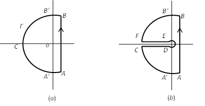
Figure 2: Contour integral of the inversion Laplace transformation
If the function \(\bar{f}(\lambda)\) is a single-valued function of \(\lambda\) with finite poles, we complete the contour by a large circle \(\Gamma\) of radius \(R\), as shown in Figure 2 \((a)\), not passing through any pole of the integrand. In the heat conduction problem governed by the equation:
(71)\[\frac{\partial T}{\partial t} = \kappa(\frac{\partial^2 T}{\partial r^2}+ \frac{1}{r}\frac{\partial T}{\partial r})\]The integral over the large circle \(\Gamma\) vanishes in the limit as \(R \rightarrow \infty\) . Thus, the contour integral is equal by Residue theorem to \(2\pi i\) times the sum of the residues at the poles of its integrand. This case usually takes place in problems on heat conduction in finite regions.
If \(\bar{f}(\lambda)\) has a branch point at \(\lambda=0\) (\(\bar{f}(\lambda)\) is multi-valued at \(\lambda=0\)). In such cases, the contour of Figure 2 \((b)\) is used with a cut along the negative real axis so that \(\bar{f}(\lambda)\) is single-valued function of \(\lambda\) within and on the contour. In the limit as the radius of the large circle tends to infinity, the integral round it can be shown to vanish and the integral in Eqn (70) is replaced by a real infinite integral, derived from the integrals along \(CD\) and \(EF\) with contributions from the small circle of radius \(R'\) about the origin and any poles of the integrand.
If the function \(\bar{f}(\lambda)\) does not belong to either of the types above, special methods must be devised to deal with it.
Note
For the details , user can check Chapter 13 in Ref.2 [2] .
| [1] | Watson: A treatise on the theory of Bessel functions. Cambridge university press (1966) |
| [2] | (1, 2, 3) Carslaw and Jaeger: Conduction of Heat in Solids, 2nd edition. Oxford University Press, Oxford, UK (1959) |