Fluid flow in porous media and Carter’s equation
Porous medium
A porous medium is a multiphase substance containing void spaces between the solid portions through which the fluid can pass. The solid portion of the substance is often called the skeleton, matrix or frame while void portions are called pores that are typically filled with fluids (liquid or gas). At least some of the pore spaces should connect each other to form networks so that fluid can flow inside the medium as shown in Figure 1. The pore network is called effective pore spaces while the disconnected ones are called ineffective pores [1] .
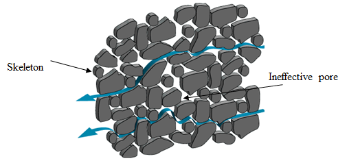
Figure 1: Fluid flows through pore networks inside a porous medium [2]
The petroleum reservoir is a natural underground geologic formation containing porous rock and fluids. The rock pores contains different types of hydrocarbons known as oil or gas in liquid or liquid-gas phase. When the engineered fluids are injected through the perforation holes to generate and propagate the fracture in the porous rock formation during hydraulic fracturing, a portion of the fluids also leaks into the porous rock formation. As a consequence, the mechanics of the fluid flow in porous media is playing a significant role to determine the fracture dimensions.
The mechanics of the fluid flow in porous media is a branch of the fluid mechanics concentrating on the fluid motion in porous media. It usually studies a portion of the porous media which is called the system of porous flow and other portions are called circumstance of porous flow as shown in Figure 2. The system of porous flow is an open system if there is free mass and energy exchange and it is a closed system if there is no free mass and energy exchange.
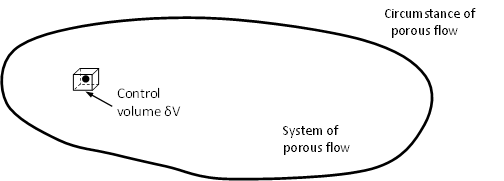
Figure 2: A control volume of a given point
A porous medium is often characterized by its porosity \(\phi\), which is the fraction of the pores volume \(V_p\). A control volume \(\delta V\) needs selecting as shown in Figure 2 before the porosity of a point is defined. The control volume cannot be neither too small (to contain sufficient effective pores) or too big (to characterize local properties of the medium), which makes \(\phi\) a continuous function on each point of the medium. If the medium is homogeneous with respect to \(\phi\), \(\phi\) can be written as:
where: \(V\) is the bulk volume of the porous medium.
The fluid equation of state
The fluid flow is generally categorized into three different types with three different fluid equation of state:
Incompressible flow
The incompressible fluid refers to the fluid in which the density of a fluid parcel (infinitesimal control volume) is independent of the pressure under the constant temperature. The equation of state can be written as:
where: \(V, p\) and \(\rho\) are the bulk volume, net pressure and density of the flow, respectively.
The incompressible fluid does not exist in the real world and it is only used to simplify some mathematical models.
Weakly compressible fluid
The weakly compressible fluid is the fluid such that the volume change is proportional to the pressure change under the constant temperature with a constant proportional coefficient known as the isothermal compressibility \(c_1\). The equation of state can be written as:
where: the constant \(\rho_0\) and \(p_0\) are the density and net pressure at a reference state.
The second equation of Eqn (3) can be rewritten as Eqn (4) by ignoring higher-order terms of its Taylor expansions:
Usually, liquid can be treated as weakly compressible fluid because the compressibilities are of order of \(10^{-4}\) . The fluid discussed in this document refers to the weakly compressible fluid, unless specified.
Compressible fluid
Compressible fluid refers to the fluid whose density changes significantly with pressure or temperature change. Gas usually behaves as compressible fluid that can be described by the real gas law:
where:
- \(p\) is the net fluid pressure, with unit [\(MPa\)]
- \(Z\) is the real gas compressibility factor, dimensionless
- \(V\) is the gas volume, with unit [\(m^3\)]
- \(V\) is the gas volume, with unit [\(kmol\)]
- \(R\) is the real gas constant, with unit [\(\frac{MPa \cdot m^3}{kmol \cdot K}\)]
- \(T\) is the gas temperature, with unit [\(K\)]
All the parameters in this document are with S.I. unit, unless specified.
And the isothermal gas compressibility is defined as:
The subscript \(T\) represents that the partial derivative is taken at constant temperature.
When \(Z=1\), the gas becomes ideal and Eqn (6) is reduced to the Boyle-Mariotte law:
The fluid equation of motion: Darcy law
The fluid equation of motion in fluid dynamics is the well-known Navier-Stokes (NS) equations, which, however, cannot be applied directly here for the fluid flow in porous media due to its non-linearity and the complex of the pores network. Some extra assumptions are needed, yielding the Darcy law.
Preliminaries
Before going to the Darcy law, some preliminary concepts need clarifying by presenting two concepts:
The velocity of fluid flow through porous media \(v\): It is the volumetric rate of the fluid flow \(Q\) passing through a unit cross-section \(A\) of the porous media:
(8)\[v = \frac{Q}{A}\]The average velocity(seepage) of fluid particle \(U\): It is defined as the volumetric rate of the fluid flow \(Q\) passing through a unit cross-section \(A_{effective}\) of the porous network:
(9)\[U = \frac{Q}{A_\mathrm{effect}}=\frac{Q}{A\phi}\]
The two concepts are illustrated in Figure 3 in which the dash arrows indicate the flow does not pass through the skeleton but he whole area is used for calculation.
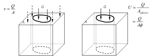
Figure 3: Velocity and seepage
It is necessary to define the seepage of the fluid particle \(U\) because the pore structure of porous media is so complicated that the velocity of one fluid particle inside is of little significance to characterize the whole fluid flow. The physical meaning of \(U\) is the average of the velocity field of a porous media control volume. The relation of \(v\) and \(U\) is:
Eqn (10) is also known as the Dupuit-Forchheimer relation.
Darcy law
The Darcy law was first deduced by Darcy as an empirical equation (Eqn (11)) to describe the one-dimensional (\(1D\)) flow for a series experiment in which he varied the amount of water flowing through a cross-sectional area \(A\) of sand filling tube as shown in Figure 4 .
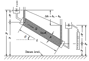
Figure 4: A schematic view of Darcy experiment [3]
The result of the Darcy experiment indicate that the volumetric rate \(Q\) of the fluid flow passing through the cross-section is proportional to the cross-section \(A\), inversely proportional to the tube length \(L\) and proportional to the piezometric head difference of the two sides of the tube (\(\triangle h = h_1-h_2\)) in a quasistatic process, which means the system passes continuously through a sequence of equilibrium states [4]
\(K\) is the hydraulic conductivity defined as:
where:
- \(k\) is the permeability of the porous media, with S.I. unit [\(m^2\)], which is a measure of the ability of porous media to allow fluids to pass through it
- \(\mu\) is the fluid viscosity, with S.I. unit [\(Pa \bullet sec\)]
For the fluid per unit mass in a quasistatic process, the energy conservation yields:
The three terms at the right-hand side of Eqn (13) represent the pressure potential, position potential energy and kinetic energy of this unit-mass fluid, respectively. And \(H\) is the Hubbert’s potential energy per unit mass of fluid. Notice that \(z\) is the elevation of the point at which the piezometric head is being considered above the datum level and has the relation with the piezometric head \(h\) :
Because the seepage is small, the kinetic term can be ignored then \(h=H\) . Then we can write \(h\) for point \(1\) and \(2\) in Figure 4 , respectively:
Since \(z_1-z_2=L\sin\theta\):
where: \(\theta\) is the inclination of the tube with respect to the horizontal datum.
Substitution of Eqn (16) and Eqn (12) into Eqn (11) :
Eqn (17) is the one-dimensional Darcy law.
The ” \(-\) “sign is due to the opposition of the velocity direction and pressure increase direction.
The differential equation of Eqn (17) is:
When the gravity is ignored, the permeability \(k\) becomes a second-rank tensor for a three-dimensional Darcy law in tensor form:
where:
- the subscripts \(i\) and \(j\) represent the coordinate components \(x\) , \(y\) and \(z\);
- the subscript comma “,” represent the partial derivative, i.e. \(p,_j=\frac{\partial p}{\partial j}\)
- it follows the Einstein summation convention that when an index variable appears twice in a single term, it implies summation of that term over all the values of the index: \(k_{ij}p,_j=k_{ix}\frac{\partial p}{\partial x}+k_{iy}\frac{\partial p}{\partial y}+k_{iz}\frac{\partial p}{\partial z}\)
The S.I. unit of the permeability is \(m^2\) while another practical unit Darcy [D] is also used in honor of the developer of the Darcy law such that \(1(D)=1(\mu m)^2\).
Continuity equation
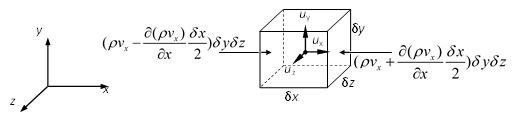
Figure 5: A control volume to derive the continuity equation
The continuity equation in fluid mechanics (Eqn (20)) is derived by considering the mass conservation for a control volume as shown in Figure 5 , in which only the flow in \(x\) direction is shown.
For the fluid flow in porous media, the effective volume for fluid flow is \(\phi \delta x \delta y \delta z\) instead of \(\delta x \delta y \delta z\), thus the continuity equation becomes:
Governing equation of one-dimensional fluid flow in a porous medium
Constant permeability and porosity
The governing equation of one-dimensional fluid flow in a homogeneous and isotropic porous medium is derived from the combination of:
The fluid equation of state (weakly compressible assumed)
(22)\[\begin{split}\left\{ \begin{align} & c_1 = -\frac{1}{V}\frac{dV}{dp} = \frac{1}{\rho}\frac{d\rho}{dp} \\ & \rho = \rho_0 [1+c_1(p-p_0)] \\ \end{align} \right.\end{split}\]The Darcy law without body force:
(23)\[v_x = -\frac{k}{\mu} \frac{\partial p}{\partial x}\]The continuity equation:
(24)\[\frac{\partial (\phi \rho)}{\partial t} = -\frac{\partial (\rho v_x)}{\partial x}\]
Substitute Eqn (23) into the right-hand side of Eqn (24):
From Eqn (22):
Substitute Eqn (26) and Eqn (22) into Eqn (25):
Substitute Eqn (27) into the left-hand side of Eqn (24):
Combine Eqn (27) and Eqn (28):
With the definition of the piezometric conductivity:
Eqn (29) can be rewritten as:
Eqn (31) is the governing equation of the 1D Newtonian laminar flow in a homogeneous isotropic porous medium by assuming the fluid is weakly compressible and the permeability and porosity are both constant.
Elastic porous medium
If the porous medium is elastic, i.e. the permeability and porosity are both functions of pressure in the similar form of the density:
where: \(k_0\) and \(\phi_0\) are constant permeability and porosity at the reference state
Then the left side of Eqn (24) becomes:
Because all the compressibilities are of order \(10^{-4}\) , Eqn (33) can be written as:
The right side of Eqn (24) becomes:
Because the term \(\frac{\partial^2 p}{\partial x^2}\) and \((\frac{\partial p}{\partial x})^2\) are of the same order, we have:
And the compressibilities are of order of \(10^{-4}\): \((c_1+c_k)(p-p_0) \ll 1\) , thus Eqn (35) can be rewritten as:
Combine Eqn (34) and Eqn (36) with introducing the total compressibility \(c_t=c_1+c_\phi\) :
And: the conductivity \(K=\frac{k_0} {\mu \rho_0 c_t}\)
Eqn (37) is the governing equation of the 1D Newtonian laminar flow in a homogeneous isotropic elastic porous medium.
To sum up, Eqn (37) and Eqn (31) can be unified by defining on the conductivity \(K\) based on the total compressibility \(c_t\).
Carter’s equation
Analytical solution to the 1D fluid flow leakoff
An element of one pressurized fracture with leakoff can be illustrated in Figure 6 . An infinite homogeneous and isotropic porous medium is located at the positive part of \(x\) axis while the interface between the medium and fracture is located at \(x=0\) (\(y\) axis), where the fluid pressure keeps constant \(p_c\) since time \(t=0\) . The fluid is leaking with velocity \(v\) through the element to the porous medium and reaches the infinity with pressure dropping to the constant pore pressure \(p_0\). At the initial time \(t=0\) , the fluid pressure within the medium is \(p_0\) everywhere.
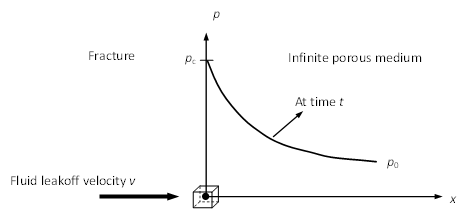
Figure 6: Schematic view of one pressurized crack with leakoff
Then, the fluid flow in the porous medium can be treated as a 1D seepage model based on the governing equation Eqn (38)
with boundary conditions and initial condition as:
The boundary conditions and initial condition are “self-similar” (see here for details), and the analytical solution is:
Derivation of the Carter’s equation
Once we get the analytical solution as Eqn (40), the leakoff velocity at the fracture/medium interface can be obtained with the following procedure:
Substitution of Eqn (41) into Darcy law Eqn (19) for 1D fluid in homogeneous and isotropic porous medium:
At the fracture/medium interface \(x=0\) , the leakoff velocity may be written with defining the pressure drop from the interface to remote \(\triangle p = p_c-p_0\) :
\(v_L\) is called leakoff velocity in hydraulic fracturing to measure how fast the fluid inside a fracture leaks to the surrounding porous medium. If it takes time \(t_0\) for the element to get exposed to the fluid, the \(t\) inside Eqn (43) should be replaced by \(t-t_0\) because this time-square-root term in the denominator represents how long the element has been exposed (\(t-t_0\)) instead of the actual time \(t\) :
Then the well-known Carter’s leakoff coefficient comes to us by [6]:
Then Eqn (44) can be rewritten as:
Eqn (46) is the Carter’s equation [6] to model the leakoff in hydraulic fracturing, which is based on the solution to 1D fluid flow in a porous medium .
| [1] | Wang Xiaodong: Basics of fluid flow in porous media. Petroleum Industry Press, Beijing, China (2006) |
| [2] | http://hercules.gcsuedu/~sdatta/home/teaching/hydro/lectures/darcy.html |
| [3] | http://www.interpore.org/reference_material/mgfc-course/mgfcdarcy.html |
| [4] | Wang: Theory of Linear Poroelasticity with Applications to Geomechanics and Hydrogeology, Princeton University Press, USA (2000) |
| [5] | Bear: Dynamics of fluids in Porous Media. American Elsevier, USA (1972) |
| [6] | (1, 2) Howard and Fast: Optimum fluid characteristics for fracture extension, API, 261-270 USA (1972) |