Wellbore Temperature Distribution¶

Governing equations¶

Equation of continuity¶

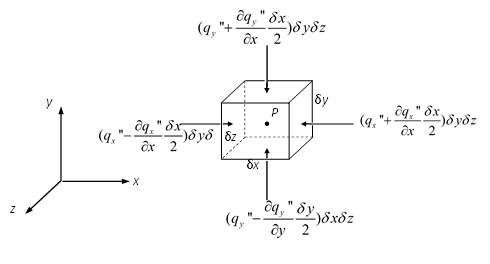
Figure 1: heat flux flowing through an infinitesimal element

Consider an infinitesimal rectangular element of a volume through which heat is flowing without heat generation inside, as illustrated in Figure 1. The temperature \(T\) at its center point \(P(x_0,y_0,z_0)\) is a continuous function of \(x,y,z\) and time \(t\), and the same is true for the heat flux \(q''\) (the rate of heat per unit area with S.I. unit \(W/m^2\)). The subscript \(x,y,z\) represent the axis direction in which the heat flows. For better visualization, the heat flux in \(z\) direction is not presented. And all the parameters in this document are with S.I. units unless specified.

From the Taylor expansion theory, the heat flux through the right surface can be expressed as:

(1)\[\begin{split}\begin{equation} \begin{split} q_\mathrm{xR}''& = q_x''(x_0+\frac{\delta x}{2}, y_0, z_0) \\ & = \sum_{n=0}^{\infty}{\frac{q_x''^{(n)}(x_0,y_0,z_0)}{n!} (x_0 + \frac{\delta x}{2}-x_0)^n} \\ & = q_x''(x_0,y_0,z_0) + \frac{\partial q_x''(x_0,y_0,z_0)} {\partial x} \frac{\delta x}{2} + \frac{\partial^2 q_x''(x_0,y_0,z_0)} {\partial x^2} (\frac{\delta x}{2})^2 + \dots \\ & \approxeq q_x'' + \frac{\partial q_x''} {\partial x} \frac{\delta x}{2} \end{split} \end{equation}\end{split}\]

where: \(q_x''\) is the heat flux in \(x\) direction at point \(P\).

The corresponding heat rate flow is: \(q_{xR} = (q_x'' + \frac{\partial q_x''}{\partial x} \frac{\delta x}{2})\delta y \delta z\)

Similarly, the heat rate flow through the left surface is: \(q_\mathrm{xL} = (q_x'' - \frac{\partial q_x''}{\partial x} \frac{\delta x}{2})\delta y \delta z\)

Then the net heat rate gain in \(x\) direction is:

(2)\[\begin{split}\begin{equation} \begin{split} \delta q_\mathrm{x}& = q_\mathrm{xL} - q_\mathrm{xR} \\ & = - \frac{\partial q_x''}{\partial x} \delta x \delta y \delta z \end{split} \end{equation}\end{split}\]

Similarly,

\[\begin{split}\left\{ \begin{align} & \delta q_y = -\frac{\partial q_y''}{\partial y}\delta x \delta y \delta z \\ & \delta q_z = -\frac{\partial q_z''}{\partial z}\delta x \delta y \delta z \\ \end{align} \right.\end{split}\]

The total net gain of the heat rate is then:

(3)\[\begin{split}\begin{equation} \begin{split} \delta q& = \delta q_x + \delta q_y + \delta q_z \\ & = - ( \frac{\partial q_x''}{\partial x} + \frac{\partial q_y''}{\partial y} + \frac{\partial q_z''}{\partial z})\delta x \delta y \delta z \\ & = - ( \frac{\partial q_x''}{\partial x} + \frac{\partial q_y''}{\partial y} + \frac{\partial q_z''}{\partial z})\delta V \end{split} \end{equation}\end{split}\]

where: \(\delta V\) is the volume of the infinitesimal element.

The net gain of heat can also be expressed as:

(4)\[\begin{split}\begin{equation} \begin{split} \delta Q& = cm \delta T \\ & = c \rho \delta V \delta T \\ \end{split} \end{equation}\end{split}\]

where:

\(c\) is the specific heat capacity, with S.I. unit [\(\frac{J}{kg \bullet K}\)]
\(\rho\) is the density of the medium through which the heat flows, with S.I. unit [\(\frac{kg}{m^3}\)]
\(T\) is the temperature, with S.I. unit [\(K\)]

Then, Eqn (3) and Eqn (4) can be related as:

(5)\[\delta q = \frac{\delta Q}{\delta t}=\rho c \frac{\partial T}{\partial t} \delta V\]

where: \(t\) is the time.

Cancellation of \(\delta V\) yields the equation of continuity in hydrodynamics without heat generated at the point:

(6)\[\rho c \frac{\partial T}{\partial t} + ( \frac{\partial q_x''}{\partial x} +\frac{\partial q_y''}{\partial y}+\frac{\partial q_z''}{\partial z})=0\]

Equation of heat transfer¶

Fourier’s law¶

The heat flux relates to the temperature gradient with the Fourier’s law:

(7)\[\begin{split}\left\{ \begin{align} & \delta q_x'' = -k \frac{\partial T}{\partial x} \\ & \delta q_y'' = -k \frac{\partial T}{\partial y} \\ & \delta q_z'' = -k \frac{\partial T}{\partial z} \\ \end{align} \right.\end{split}\]

Or in a more concise form:

(8)\[q_i'' = -kT,_i\]

where:

the subscripts \(i\) represent the coordinate components \(x\) , \(y\) and \(z\);
the subscript comma “,” represent the partial derivative, i.e. \(T,_i=\frac{\partial T}{\partial i}\)

Substitute Eqn (7) into Eqn (6):

(9)\[\rho c \frac{\partial T}{\partial t} - [ \frac{\partial}{\partial x}(k \frac{\partial T}{\partial x}) +\frac{\partial}{\partial y}(k \frac{\partial T}{\partial y}) +\frac{\partial}{\partial z}(k \frac{\partial T}{\partial z})] =0\]

where: \(k\) is the heat conductivity with S.I. unit [\(\frac{W}{m\bullet K}\)]

Eqn (9) is the equation of heat conduction without internal heat generation.

If the heat conduction medium is homogeneous and isotropic, \(k\) is then independent of position, reducing Eqn (9) to:

(10)\[\rho c \frac{\partial T}{\partial t} - k(\frac{\partial^2 T}{\partial x^2} + \frac{\partial^2 T}{\partial y^2} \frac{\partial^2 T}{\partial z^2}) =0\]

Introducing the Laplace operator \(\nabla^2 \equiv \frac{\partial^2}{\partial x^2} +\frac{\partial^2}{\partial y^2}+\frac{\partial^2}{\partial z^2}\), Eqn (10) can be rewritten as a concise form:

(11)\[\frac{\partial T}{\partial t}=\kappa \nabla^2 T\]

where: \(\kappa = \frac{k}{\rho c}\) represents the thermal diffusivity, with S.I. unit [ \(m^2/s\)] .

Internal heat generation¶

The above derivation excludes the internal heat generation. If the rate of the heat generated internally per unit volume is denoted by \(\phi (\frac{W}{m^3})\), Eqn (3) becomes:

(12)\[\delta q = - ( \frac{\partial q_x''}{\partial x} + \frac{\partial q_y''}{\partial y} + \frac{\partial q_z''}{\partial z})\delta V + \phi \delta V\]

Equating Eqn (12) and Eqn (5) obtains the heat conduction equation with internal heat generation:

(13)\[\frac{\partial T}{\partial t}=\kappa \nabla^2 T + \frac{\phi}{\rho c}\]

Moving medium (convective component)¶

An even more general heat transfer equation without radiation also takes account of the effect of the relative motion between the material system and the coordinate with a velocity \(v\). Then the convective term of components must be added to the heat flux:

(14)\[q_i'' = -kT,_i + \rho c T v_i\]

Substitute Eqn (14) into Eqn (6):

(15)\[\frac{\partial T}{\partial t} + v_x \frac{\partial T}{\partial x} + v_y \frac{\partial T}{\partial y} + v_z \frac{\partial T}{\partial z} =\kappa \nabla^2 T + \frac{\phi}{\rho c}\]

Notice that \(v_x = \frac{\partial x}{\partial t}\) etc. Eqn (14) can be rewritten in a more concise form:

(16)\[\frac{DT}{Dt}=\kappa \nabla^2 T + \frac{\phi}{\rho c}\]

With the definition of the total derivative:

(17)\[\frac{DT(x,y,z,t)}{Dt} \equiv \frac{\partial T}{\partial t} + \frac{\partial T}{\partial x}\frac{\partial x}{\partial t} + \frac{\partial T}{\partial y}\frac{\partial y}{\partial t} + \frac{\partial T}{\partial z}\frac{\partial z}{\partial t}\]

Equation of heat transfer in Cylindrical coordinate¶

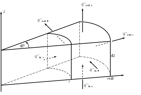
../_images/infinitesimal-element-cylindrical.png

Figure 2: heat flux flowing through an infinitesimal cylindrical element

Apply the Laplace operator defined in Cylindrical coordinate as Eqn (18) \((r,\theta, z)\) as shown in Figure 2 to Eqn (16).

(18)\[\nabla^2 \equiv \frac{1}{r}( r \frac{\partial}{\partial r} + \frac{1}{r^2} \frac{\partial^2}{\partial \theta^2} + \frac{\partial ^2}{\partial z^2})\]

The explicit form of heat transfer equation Eqn (16) is then:

(19)\[\frac{\partial T}{\partial t} + v_r \frac{\partial T}{\partial r} + \dot \theta \frac{\partial T}{\partial \theta} + v_z \frac{\partial T}{\partial z} =\kappa [ \frac{1}{r}( r \frac{\partial T}{\partial r} + \frac{1}{r^2} \frac{\partial^2 T}{\partial \theta^2} + \frac{\partial ^2 T}{\partial z^2}) ] + \frac{\phi}{\rho c}\]

Note

Eqn (16) is the concise form of heat transfer governing equation excluding radiation for both Cartesian and Cylindrical coordinate. Eqn (15) and Eqn (19) are the explicit forms for the two different coordinates.

Wellbore temperature distribution¶

Problem statement and Ramey solution¶

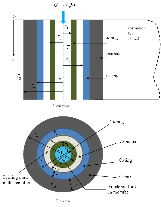
Figure 3: A schematic view of a wellbore

A typical wellbore transient heat transfer problem is illustrated in Figure 3 with the wellbore axis coinciding with \(z\) axis so that the system is axisymmetric (\(\theta\) is irrelevant). The fluid with initial temperature \(T_0\) is injected downhole with constant volumetric rate \(Q_0\) and the fluid temperature inside tubing \(T_1(r,z,t)\) and the formation temperature \(T_2(r,z,t)\) need solving.

The system consists of three different parts from inside to outside of the wellbore:

Fluid-flow conduit inside the tubing represented by the subscript \(t\): \(0 \leqslant r < r_1\);
Tubing, casing annulus, casing and cement represented by the subscripts \(t, c, a\) and \(ce\), respectively: \(r_1 \leqslant r \leqslant r_w\);
Infinite horizontally layered formation surrounding the case: \(r> r_w\).

And:

\(h\) represents the heat conductivity, heat transfer coefficient [\(\frac{W}{m^2 \bullet K}\)];
\(x\) is the thickness here.

In addition, some assumptions are made as follows so that an analytical solution or approximation can be obtained [1]:

The formation is homogeneous and isotropic;
The properties of the fluid and formation are constant;
Fluid in the tube flows with a constant flow rate \(Q_0\) in the direction of the wellbore only;
The heat conduction in the system is only radial;
Steady radial heat flow is assumed inside the wellbore-formation interface (\(0 \leqslant r \leqslant r_w\)), hence it can be represented by a single steady-state heat transfer coefficient \(U\). [1] [2] ;
The fluid temperature inside the tubing is lumped radially (\(T_1\) is the same for for \(0 \leqslant r \leqslant r_1\) at the same \(z\)) so that \(T_1\) is only the function of \(z\) and \(t\) : \(T_1(z,t)\);
The initial formation temperature distribution is a known function of depth \(T_e(z)\) (initial condition);
The temperature at far away satisfies the known function \(T_e(z)\) ( boundary condition);
The surface fluid temperature is kept at \(T_0\).

Table-1: Nomenclature table for Ramey solution¶
Parameter	unit	Parameter	unit
Geothermal gradient \(a\)	\(\frac{^{\circ}F}{ft}\)	mass flow rate \(W\)	\(\frac{lb}{min}\)
Surface geothermal temperature \(b\)	\(^{\circ}F\)	Specific heat at constant pressure of fluid \(c\)	\(\frac{Btu}{lb \bullet ^{\circ}F}\)
Surface temperature of injected fluid \(T_0\)	\(^{\circ}F\)	Earth thermal conductivity \(k\)	\(\frac{Btu}{hr \bullet lb \bullet ^{\circ}F}\)
Wellbore length \(L\)	\(ft\)	Earth thermal diffusivity \(\alpha\)	\(\frac{ft^2}{hr}\)
Vertical depth \(H\)	\(ft\)	Time function \(f(t)\)	dimensionless

With the introduction of the parameters given in Table 1, the Ramey solution is given to predict the temperature at the depth \(z\) as shown in Figure 3 :

(20)\[T_1 = az+b-aA+(T_0+aA-b)e^{-\frac{z}{A}}\]

where: the function \(A\) is defined as:

(21)\[A = \frac{Wc[k+r_1Uf(t)]}{2 \pi r_1 Uk}\]

Then, the formation temperature \(T_2\) can be found based on the three different boundary conditions listed in Figure 4 [1].

The derivation can be seen here.

The overall thermal coefficient \(U\) can be assumed infinite (negligible wellbore thermal resistance) when a liquid is injected down casing [1], resulting in a simplified \(A\) :

(22)\[A = \frac{Wcf(t)}{2 \pi k}\]

The time function \(f(t)\) can be read from Figure 4 as given in the literature [1] . The \(r_2'^2\) in the figure is the \(r_w\) in Figure 3.

Figure 4: The time function

The steady heat flow inside wellbore assumption can be satisfied well when the dimensionless time \(t_D = \frac{\alpha t}{r_w^2}\) is large, making Ramey solution quite accurate for the long injection time. At the early time or short injection time (like a couple hours for hydraulic fracturing) when \(t_D\) is small, the Ramey solution does not match the results obtained numerically as accurately as for the large \(t_D\) [3] [4] [5]. However, the fluid flow downhole temperature \(T_1\) does not vary as much as other parameters, e.g. the wellbore/formation interface temperature, when comparing with the numerical ones [3]. Thus, the Ramey solution is still a good benchmark for the fluid downhole temperature in wellbore heat transfer problems.

Example calculation¶

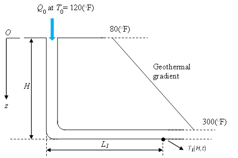
Figure 5: Schematic view of the Ramey solution application

A sample calculation can be made based on the schematic view as shown in Figure 5. The data can be given as follows [1]:

The volumetric flow rate \(Q_0=100(bbl/min)\)
No tubing so that the inner radius of the wellbore \(r_1=3.183(in)\), and the outer radius \(r_c=3.5(in)\)
The vertical height \(H=10^4(ft)\) and the horizontal length \(L_1=10^4(ft)\), thus the total length \(L = H+L_1 = 2 \times 10^4(ft)\)
The geothermal temperature is given by: \(80+0.022z(^{\circ}F)\), thus the geothermal gradient \(a = 0.022(\frac{^{\circ}F}{ft})\) and the surface geothermal temperature \(b = 80(^{\circ}F)\). Taking \(z = H = 10^4(ft)\), the reservoir temperature at the depth \(10^4(ft)\) is \(T_2(H,t)=300(^{\circ}F)\)
The surface temperature of the fluid \(T_0 = 120(^{\circ}F)\)
The injection time \(t_{inj} = 3(hr)\)
Assume the fracking fluid as the slick water made up of \(98\% - 99.5\%\) water in volume, whose thermal properties may be approximated with the ones of water: \(c = 1 (\frac{Btu}{lb\bullet ^{\circ}F})\)
The earth thermal conductivity \(k = 1.4 (\frac{Btu}{hr \bullet lb \bullet ^{\circ}F})\) and the earth thermal diffusivity \(\alpha = 0.04 (\frac{lb}{hr})\)

The mean velocity is:

\[v = \frac{Q}{A}=\frac{100 \times 5.61453}{\pi(3.183 \times \frac{1}{12} )} [\frac{ \frac{bbl}{min}\times \frac{ft^3}{bbl} }{ in \times \frac{ft}{in} }] = 2.5401 \times 10^3(\frac{ft}{min})\]

The time it takes for the fracking fluid to reach the destiny point:

\[t = \frac{L}{v} = \frac{2\times 10^4}{2.5401 \times 10^3} = 7.87 \approx 8 (min)\]

Then the dimensionless time \(t_D\) is [1] :

\[t_D = \frac{\alpha t}{r_c^2} = \frac{0.04 \times \frac{8}{60}} {(\frac{3.5}{12})^2} [ \frac{ \frac{ft^2}{hr} \times min \times \frac{hr}{min} } { (in \times \frac{ft}{in})^2 } ] = 0.0627\]

From Figure 5, \(\log_{10}(t_D)=-1.2028\). Because negligible thermal resistance is assumed, the constant temperature source curve should be used. Thus, the corresponding \(\log_{10}[f(t)]=-0.43\) and hence \(f(t)=0.3728\). Then the function \(A\) can be evaluated as:

(23)\[\begin{split}\begin{equation} \begin{split} A& = \frac{Wcf(t)}{2 \pi k} \\ & = \frac{ 100 \times 350 \times 1 \times 0.3728 } { 2 \pi \times 1.4 \times \frac{1}{60} } [ \frac{ \frac{bbl}{min} \times \frac{lb}{bbl} \times \frac{Btu} {lb \bullet ^{\circ}F} } { \frac{Btu}{hr \bullet lb \bullet ft \bullet ^{\circ}F} \times \frac{hr}{min} } ] \\ & = 8.899 \times 10^4 \\ & \approx 8.9 \times 10^4(ft) \end{split} \end{equation}\end{split}\]

Substitute Eqn (23) into Eqn (20):

(24)\[\begin{split}\begin{equation} \begin{split} T_1& = aH + b - aA + (T_0+aA-b)e^{-\frac{H}{A}} \\ & = 0.022 \times 10^4 + 80 - 0.022 \times 89 \times 10^4 +(120+0.022 \times 8.9 \times 10^4 -80)e^{-\frac{10^4} {8.9 \times 10^4}} \\ & = 127.66 (^{\circ}F) \end{split} \end{equation}\end{split}\]

If two different time \(t=20(min)\) and \(3(hr)\) (the injection time) are considered, the results can be obtained in a similar manner as presented in Table 2 :

Table-2: Results for different time¶
Time (min)	8	20	180
Temperature \(T_1(^{\circ}F)\)	\(127.66\)	\(125.55\)	\(122.47\)

From the results in Table 2, the fluid flow downhole temperature does not vary much from the initial surface fluid temperature (\(120 ^{\circ}F\) in this example). A uniform fluid temperature distribution along the wellbore is reasonable for the hydraulic fracturing simulation.

[1]	(1, 2, 3, 4, 5, 6, 7) Ramey: Wellbore heat transmission, JPT, 427-435 (April 1962)

[2]	Willhite: Over-All heat transfer coefficients in steam and hot water injection wells, JPT, 607-615 (May 1967)

[3]	(1, 2) Moradi, Awang: Heat transfer in the formation, SPE, 6 (21), 3927-3932 (2013)

[4]	Hagoort: Ramey’s wellbore heat transmission revisited, JPT, 465-474 (August 2004)

[5]	Wu, Pruess: An analytical solution for wellbore heat transmission in layered formations, SPERE, 531-538 (November 1990)