Reservoir Formation
Introduction
The Reservoir Formation panel is where the user can specify the geological structure of the reservoir, such as the stress distribution, temperature distribution, pore pressure, rock interface locations and rock properties. On the left side of are sub panels to input data, as well as controls for the plot. On the right is a collection of plots, one for each set of data, as shown in Figure 1.
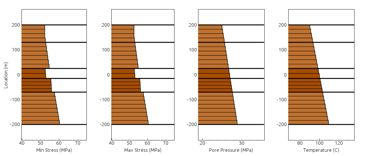
Figure 1: Example reservoir plot
Interface
The top portion of the Interface subpanel contains 3 pieces of information about the reservoir (Figure 2):
- Reference Depth: The depth at which the horizontal section of the wellbore resides. This depth is used in the simulation to help identify the most important layer.
- Element Size Along Layer: The size of a simulation elements along the layers horizontally.
- Element Size Across Layer: The size of a simulation elements across the reference layer (vertically). The element size across the layer is shown in the visualizations.
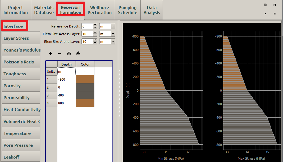
Figure 2: Interface inputs for reservoir formation
Note
- The vertical element sizes for non-reference layers are modified slightly so the element size for each element in a layer is uniform. The user can see the computed element size for each layer on the plot.
- Refined elements with smaller dimensions can provide more accurate results, but this decreases the computational efficiency. An appropriate element size should be chosen according to the scale of specific problems.
Stress
The Stress table defines the in-situ stress of the rock formation that the induced hydraulic fracture needs overcome to propagate. The Depth column defines the location where the stresses are applied. The Min stress is the minimum horizontal stress, denoted by \(\sigma_\textrm{h,min}\) , which may be expressed as [1] :
where:
- \(\nu\) is the Poisson’s ratio
- \(g\) is the gravity acceleration constant, about 9.81 \(\mathrm{m}/\mathrm{s}^2\)
- \(\alpha\) is the poroelastic constant
- \(p\) is the pore pressure
- \(\sigma_{\nu}\) is the absolute vertical stress (simply the weight of the overburden)
- \(\rho\) is the density of the overlaying strata
- \(H\) is the depth
In hydraulic fracture mechanics, a fracture propagates in the direction perpendicular to the one of the minimum horizontal stress \(\sigma_\textrm{h,min}\) as shown in Figure 3
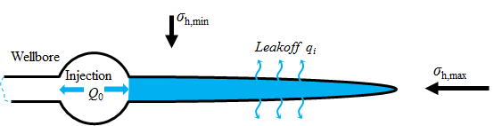
Figure 3: Schematic view of in-situ stresses
Tectonic phenomena may result in an additional horizontal in-situ stress component \(\sigma_\textrm{tect}\) and thus the other horizontal in-situ stress is larger than \(\sigma_\textrm{h,min}\) [1]. This stress is called maximum horizontal stress \(\sigma_\textrm{h,max}\) and may be expressed as:
The Max Stress in the Stress subpanel represents \(\sigma_\textrm{h,max}\).
In FrackOptima, the user simply inputs the minimum and maximum horizontal stresses, without considering the details of the equations given above. The difference of the two stresses is typically a couple of \(\textrm{MPa}\). For example \(\textrm{3MPa}\) is enough for a PKN model to contain the fracture height [2]. A reasonable pair inputs may be \(\sigma_{h,min}=\textrm{30 MPa}\) , and \(\sigma_{h,max}=\textrm{33 MPa}\).
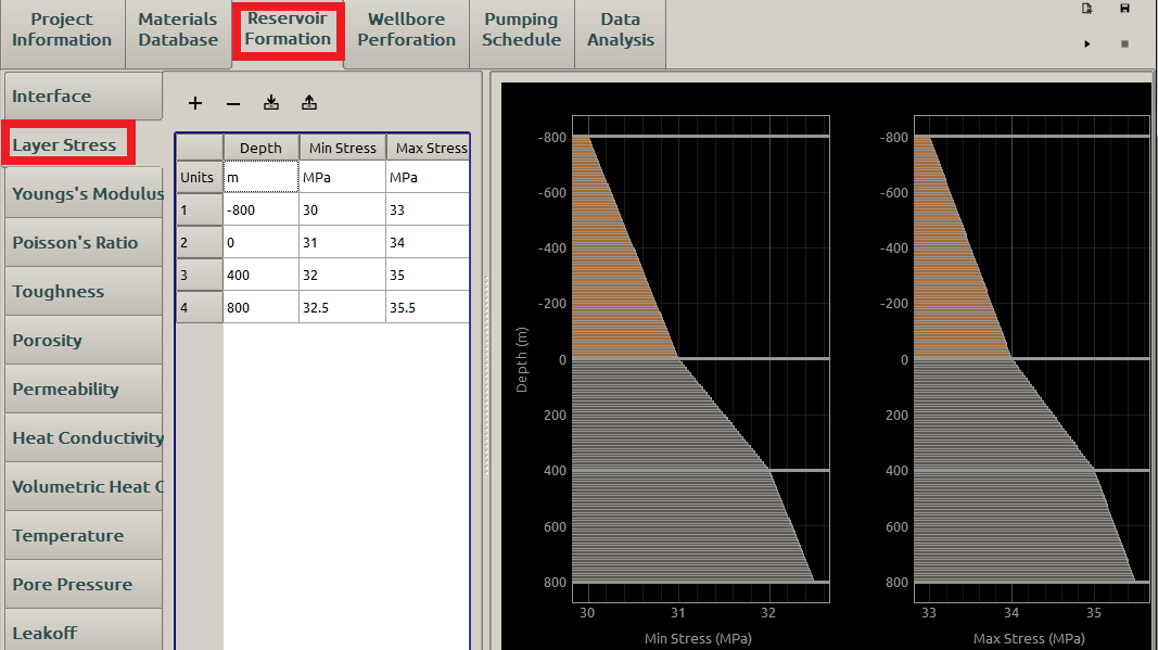
Figure 4: Interface inputs for stress profile
Young’s Modulus
Young’s Modulus, usually denoted as \(E\), is a measure of the stiffness of an elastic material and characterizes the material’s ability to resist deformation under load. It is the slope of the stress vs strain curve for a material with linear elastic deformation, as shown in Figure 5. Typical values of Young’s modulus for rock formations ranges from a couple of \(\textrm{GPa}\) to about 40 \(\textrm{GPa}\) [3] .
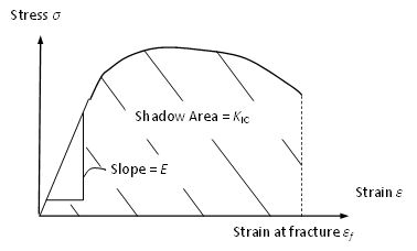
Figure 5: A schematic stress-strain curve
If an invalid value is given for Young’s modulus, the value will be highlighted red as shown in Figure 6. The same error indicator appears if an invalid input is made by users for any other inputs.
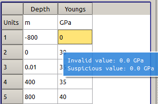
Figure 6: Invalid input indicator
If an input for the Young’s modulus is too small, say \(\textrm{0.001GPa}\), a warning appears showing the user the value is suspicious (but not totally invalid), as shown in Figure 7.
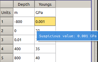
Figure 7: Suspicious input indicator
A reasonable young’s modulus input may be displayed in Figure 8 with Combine Similar Elastic Layers as False:
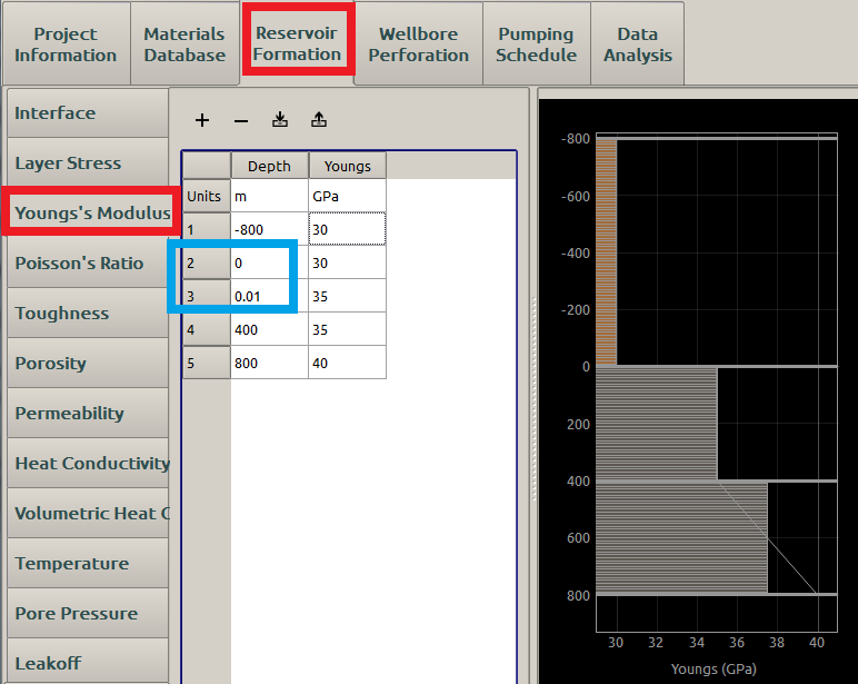
Figure 8: Input of Young’s modulus
If the Young’s modulus is not defined uniformly in a single user-defined layer, a linear extrapolation will be implemented as shown in the third layer in Figure 8. Then the average value \(\textrm{37.5 GPa}\) will be used.
Please notice that, the Combine Similar Elastic Layers in Advanced Control Parameters will affect the Young’s modulus input. Click here for details.
Last, If an instantaneous Young’s modulus jump is expected, it is best to increase the depth of the second stress by some small value, like \(\textrm{0.01 m}\) for example (blue box in Figure 8).
Poisson’s Ratio
When a material is compressed or stretched in one direction, it usually expands or contracts in the other two directions perpendicular to the direction of compression or elongation. This phenomenon is called Poisson effect, which is illustrated in Figure 9.
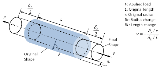
Figure 9: The scheme of Poisson effect
Poisson’s ratio, denoted by \(\nu\), is a dimensionless parameter that measures this effect. It is defined as axial strain divided by transverse strain. A typical value of \(\nu\) is 0.25 for most rock formations [3] .
A reasonable Poisson’s Ratio input may be displayed in Figure 10 :
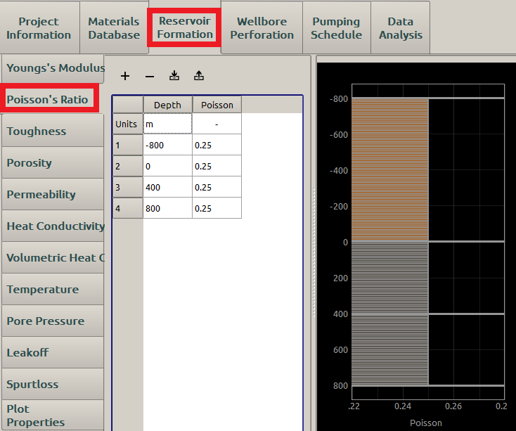
Figure 10: Input of Poisson’s ratio
Similar linear extrapolation will be implemented if the Poisson’s Ratio is not uniformly defined in a layer, similar to Figure 8.
Note
Both Young’s Modulus and Poisson’s Ratio are assumed constant in a single layer. Other parameters, e.g. Toughness etc., can be functions of the depth.
The Combine Similar Elastic Layers in Advanced Control Parameters will affect the Poisson ratio input. Click here for details.
Toughness
The rock Toughness, denoted as \(K_{IC}\), is derived from the stress intensity factor \(K\). The stress intensity factor characterizes amplification of stress at a crack (fracture) tip. The magnitude of \(K\) depends on the material’s properties, the fracture geometry, the size and location of the fracture, and the magnitude and distribution of loads. It is used to predict the stress state near the tip of a pre-existing crack in fracture mechanics. The stress distribution near the crack tip in a linear elastic medium is given by Eq. (3) in terms of \(K\) and \(\theta\) as shown in the Figure 11:
where \(f_{ij}\) is a dimensionless function that depends on the load and geometry.
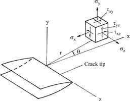
Figure 11: Stress state near the crack tip
The minimum value of \(K\) can be determined for tensile fractures, which is the predominant type of fracture in hydraulic fracturing, in plain strain conditions. The minimum value of \(K\) is the critical value required to propagate the pre-existing crack. This critical value, denoted as \(K_{IC}\), is the fracture toughness of a material, which describes the ability of a material containing pre-existing defects to resist fracture propagation while being deformed. \(K_{IC}\) may be obtained as the area below the stress-strain curve, as shown in Figure 5, before fracture occurs. In hydraulic fracturing, the fracture is assumed to propagate once the stress intensity factor \(K\) gets larger than the fracture toughness \(K_{IC}\). Some measured fracture toughness values are listed in Table 1 for various rock formations [3] .
| Formation type | \(K_{IC} (\mathrm{kPa} \bullet \sqrt{\mathrm{m}})\) | \(K_{IC} (\mathrm{psi} \bullet \sqrt{\mathrm{in}})\) |
|---|---|---|
| Siltstone | \(1048 \sim 1810\) | \(950 \sim 1650\) |
| Sandstone | \(440 \sim 1760\) | \(400 \sim 1600\) |
| Limestone | \(440 \sim 1040\) | \(400 \sim 950\) |
| Shale | \(330 \sim 1320\) | \(300 \sim 1200\) |
A reasonable Toughness input may be displayed in Figure 12 :
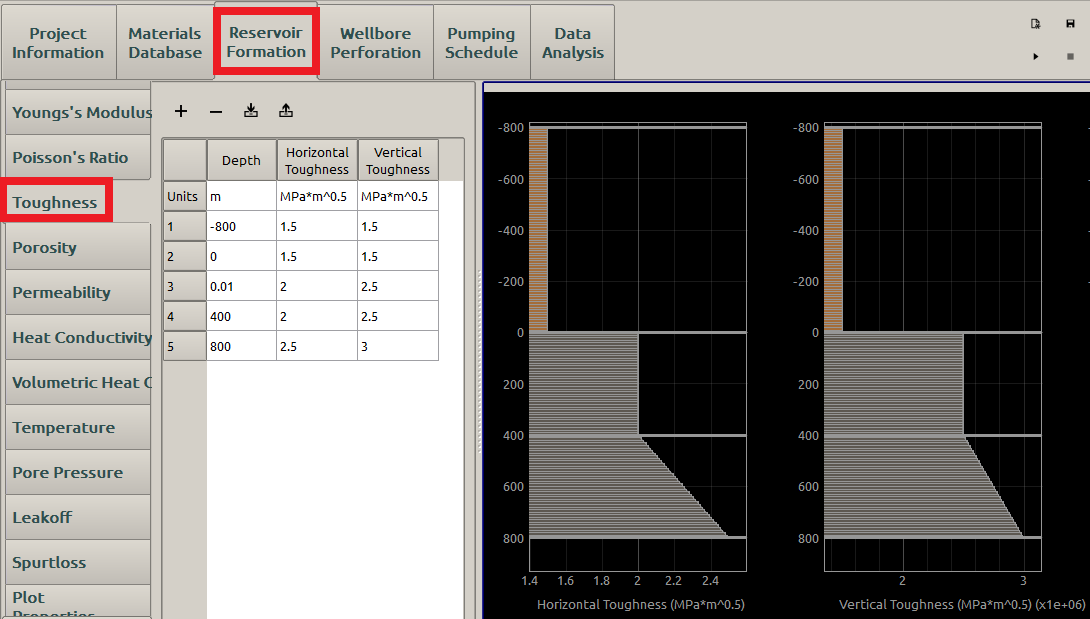
Figure 12: Input of toughness
If the input is not uniform in one layer, a direct linear extrapolation (Figure 12) is implemented but without average value used as in Young’s modulus (Figure 8) and Poisson’s ratio. This direct linear extrapolation will be used for all the following parameter inputs.
Porosity
Porosity, denoted by \(\phi\), is a fractional measure of void spaces, also known as pores, in a porous material. The void spaces (pores) may contain gas or liquids. Porosity is defined by the equation:
where: \(V_v\) and \(V\) are the void-space volume and the bulk volume, respectively.
Typical values of porosity for a rock formation may range from 0.02 to 0.5 [4] .
A reasonable Porosity input may be displayed in Figure 13 :
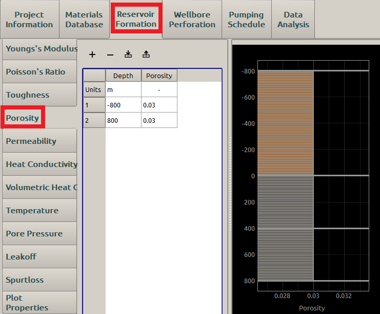
Figure 13: Input of porosity
Permeability
The Permeability, usually denoted by \(k\), characterizes a material’s ability to allow a gas or fluid to pass through its pores when subjected to a pressure gradient. It is part of the proportionality constant in Darcy’s law (see here for details) which relates the leakoff flow rate and fluid physical properties, e.g. viscosity, to the pressure gradient, as in Eq. (5):
where:
- \(q_i\) is the leakoff flux (flow rate per unit area), \(\textrm{m/s}\)
- \(\nabla p\) is the pressure gradient, \(\textrm{Pa/m}\)
- \(\mu\) is the fluid viscosity, \(\textrm{Pa} \bullet \textrm{s}\)
Although the SI unit of permeability is \(\mathrm{m}^2\), the Darcy, \(\textrm{D}\), or millidarcy, \(\textrm{mD}\), is more common in petroleum industry since the rock formations deep beneath the earth surface are not very porous. One Darcy is approximately \(10^{-12} \mathrm{m}^2\). The permeability of oil reservoir rocks ranges between hundreds of \(\textrm{mD}\) to thousands of \(\textrm{mD}\) [5].
A reasonable Permeability input may be displayed in Figure 14 :
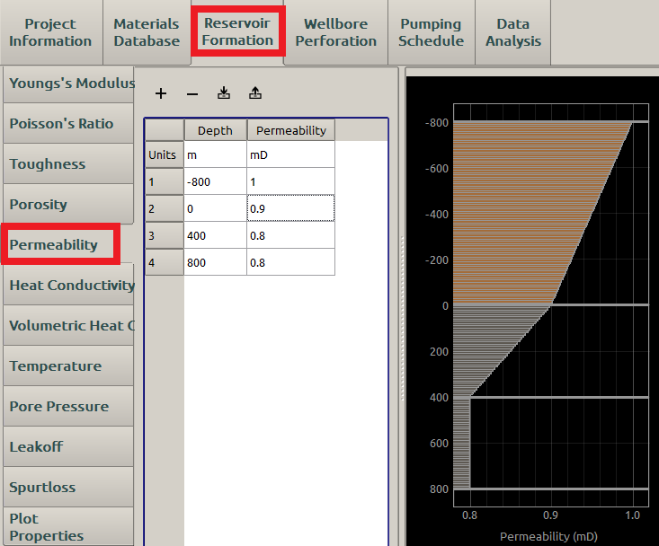
Figure 14: Input of permeability
Heat Conductivity
Heat Conductivity, also known as thermal conductivity, characterizes a material’s ability to conduct heat when subjected to temperature gradient. It is the proportionality constant, denoted as \(\lambda\), in Fourier’s law for heat conduction, shown in Eq. (6) :
where:
- \(\varphi\) is the heat flux, \(\textrm{W}/\textrm{m}^2\)
- \(\nabla T\) is the temperature gradient, \(\textrm{K/m}\)
- The minus sign “-” means the heat flux always flows from the warmer area (higher temperature) to the colder one (lower temperature).
The heat conductivity of non-metals may be assumed to be constant in the temperature range in hydraulic fracturing [6]. The heat conductivities for some rock formations at room temperature (about \(\textrm{300 K}\)) are listed in Table 2 [4] [7]:
| Formation type | \(\lambda\) (W/(m \(\bullet\) K)) |
|---|---|
| Sandstone | \(1.83 \sim 3.9\) |
| Limestone | \(1.26 \sim 1.33\) |
A reasonable Heat conductivity input may be displayed in Figure 15 :
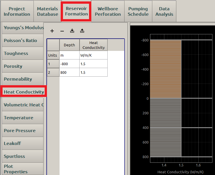
Figure 15: Input of heat conductivity
Volumetric Heat Capacity
Volumetric heat capacity, usually denoted as \(c_v\), characterizes the ability of a given volume of a substance to store internal energy while undergoing a given temperature change, but without undergoing a phase change. Some typical values for \(c_v\) are listed in the Table 3 [8] [9]:
| Formation type | \(c_v\) (\(\mathrm{J/(K \bullet m^3)}\)) |
|---|---|
| Sandstone | \(2.02\times10^6 \sim 2.58\times10^6\) |
| Limestone | \(2.09\times10^6 \sim 2.45\times10^6\) |
A reasonable Volumetric Heat Capacity input may be displayed in Figure 16 :
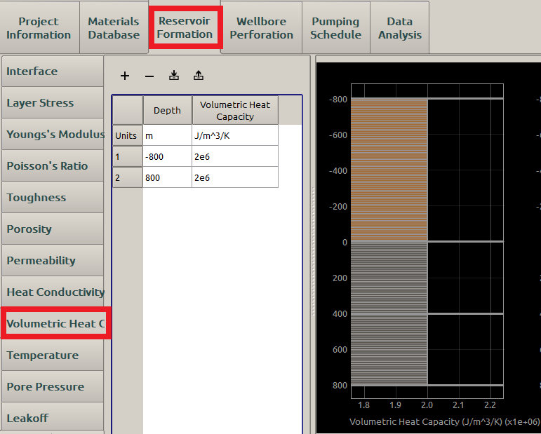
Figure 16: Input of volumetric heat capacity
Temperature
The temperature of the formation increases as the depth increases. A linear geothermal gradient is assumed in FrackOptima. Thus, the temperature in the reservoir is uniquely defined by the surface Temperature and the reservoir Temperature (at the bottom) are defined automatically as shown in Figure 17.
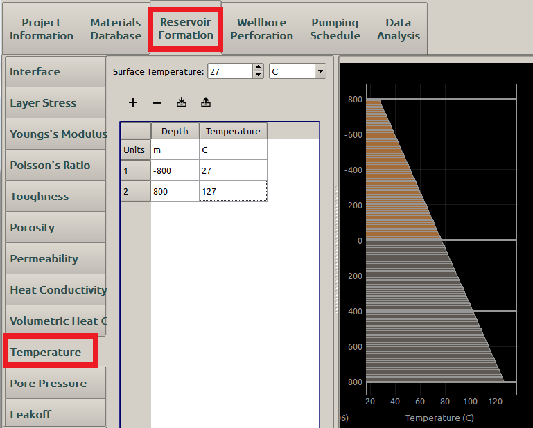
Figure 17: Temperature inputs
Note
We have determined that more complex temperature profiles have very little effect on the temperature of the fluid. The most important parts of the temperature profile are the fluids starting temperature, and the temperature in the reservoir. The temperature of the fluid changes very little before it reaches the fracture. (see here for example)
Pore Pressure
Pore pressure is the pressure of fluids within the pores of a reservoir, and is usually hydrostatic pressure or the pressure exerted by a column of water from the formation’s depth to sea level [10].
In FrackOptima, the Reference Pore Pressure, denoted as \(p_0\), is the pore pressure at the Reference Depth. A linear pore pressure profile \(p\) is assumed:
where:
- \(\rho_{res}\) is the reservoir fluid Density
- \(H\) is the depth
- \(H_0\) is the Reference Depth
Typical values of pore pressure are around \(\textrm{20 MPa}\), respectively [11]. A pore pressure profile may be displayed as Figure 18.
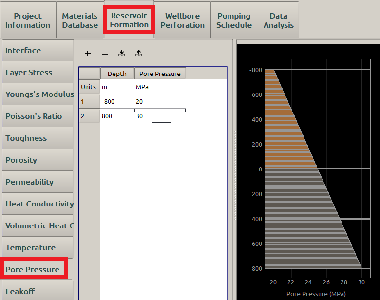
Figure 18: Pore-pressure inputs
When the Reservoir Fluid Density is set to zero, the pore pressure is distributed uniformly in the formation, as shown here.
Leakoff
Rock formations are a porous media, so the injected fracking fluid leaks off from the induced hydraulic fracture to the surrounding formation. This reduces the fluid pressure to generate and maintain the fracture. Thus, the leakoff is a key factor in determining the fracture dimensions. FrackOptima adopts the well-accepted Carter’s leakoff model, which can be expressed as [1]:
where:
- \(v_L\) is the leakoff velocity, m/s
- \(\textrm{t}\) is time
- \(\textrm{t}_0\) is time at which the fracture gets exposed to the fracking fluid. Thus \(\textrm{t}-\textrm{t}_0\) represents the duration of the fracture exposure
- \(c_L\) is Carter’s leakoff coefficient, \(\textrm{m}/\sqrt{\textrm{s}}\)
Because \(c_L\) is determined from the properties of both the rock formation and the fracking fluid, a user needs to define the fluid as marked in a red box in Figure 19.
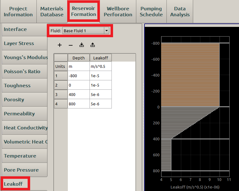
Figure 19: Inputs of leakoff coefficient
A typical value of \(c_L\) is in the range \(10^{-6} \sim 10^{-5} \mathrm{m}/\sqrt{\mathrm{s}}\) and may be smaller than that [12]. If all \(c_L\) are set as 0, the rock formation is considered as impermeable.
Spurtloss
Integration of Eq. (8) with respect to \(\textrm{t}\) yields:
where:
- \(V_L\) is the fracking fluid volume passing (leaking) through the surface \(A_L\) during the time period from \(t_0\) to \(\textrm{t}\)
- \(S_p\) is the spurtloss coefficient, which can be considered as the width of the fracking fluid body that passes through the surface instantaneously at the very beginning of the leakoff process.
Typical value of \(S_p\) is in the range \(\mathrm{10}^{-3} \mathrm{mm}\), and can be taken as 0. A set of spurtloss coefficients are shown in Figure 20 with no spurt loss.
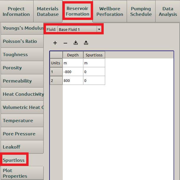
Figure 20: Inputs of spurtloss coefficient
Plot Properties
The Plot Properties subpanel is displayed as Figure 21.
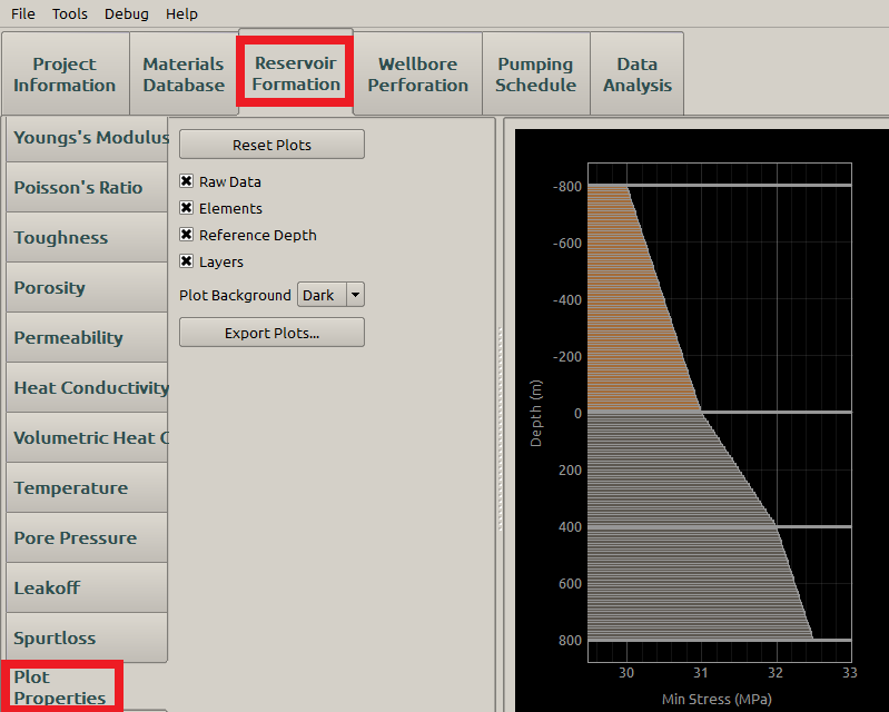
Figure 21: Plot Properties subpanel
This subpanel holds the controls for the plot. The three check boxes specify what is visible on each plot:
- Raw Data: This is the interpolated data from what the user provides from the preceding tables. Note that it is hard to see the raw data when the elements are plotted.
- Elements: Show the elements that will be used by the simulation. The size of each element can be changed with the Element Size Across Layer property. The length of the element corresponds to its value on the x-axis.
- Layers: This shows bold, horizontal lines where the interface for each layer is located.
If any of the three boxes is unchecked, the corresponding objective is not displayed at right. See Figure 22 for the Layers unchecked.
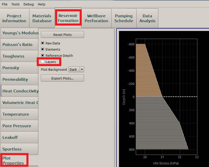
Figure 22: Plot Properties subpanel
The Plot Background drop down menu changes the background color of the plot.
The Export button will query the user for a directory in which to save all of the plots. In that directory, a new directory with the current project name will be created. Each individual plots and the composite plot will be exported to separate image files.
See also
- Importing and Exporting
- For more information on exporting plots.
| [1] | (1, 2, 3) Valko, Economides: Hydraulic Fracture Mechanics. Wiley, Chichester, UK (1995) |
| [2] | Yew: Mechanics of Hydraulic Fracturing. Gulf Publishing Company, Houston, USA (1997) |
| [3] | (1, 2, 3) Meyer 2013 User’s Guide |
| [4] | (1, 2) McLin, etc., Geochemical modeling of water-rock-proppant interactions, Geo- thermal Reservoir Engineering (2011) |
| [5] | http://en.wikipedia.org/wiki/Permeability_(earth_sciences) |
| [6] | http://en.wikipedia.org/wiki/List_of_thermal_conductivities#cite_note-Marble-Institute-52 |
| [7] | http://www.engineeringtoolbox.com/thermal-conductivity-d_429.html |
| [8] | http://www.engineeringtoolbox.com/specific-heat-solids-d_154.html |
| [9] | http://geology.about.com/cs/rock_types/a/aarockspecgrav.html |
| [10] | http://www.glossary.oilfield.slb.com/en/Terms/p/pore_pressure.aspx |
| [11] | http://www.engineeringtoolbox.com/liquids-densities-d_743.html |
| [12] | P. Valko, M. J. Economides: Propagation of hydraulically induced fractures-a continuum damage mechanics approach, Int. J. Rock Mech. Min. Sci & Geomech. Absr. 31(3), 221-229 (1994) |