PKN Hydraulic Fracturing Model
Introduction
The Perkins-Kern-Nordgren (PKN) model is another well-known 2D classic hydraulic fracturing model with a long fracturing length (hundreds of meters in length, x-axis as shown in Figure 1), limited but constant height (tens of meters in y-axis) and small width (measurable in millimeters in z-axis) propagated in an infinite homogeneous isotropic linear elastic formation characterized by Young’s modulus \(E\), Poisson’s ratio \(\nu\) and toughness \(K_{Ic}\). [1]
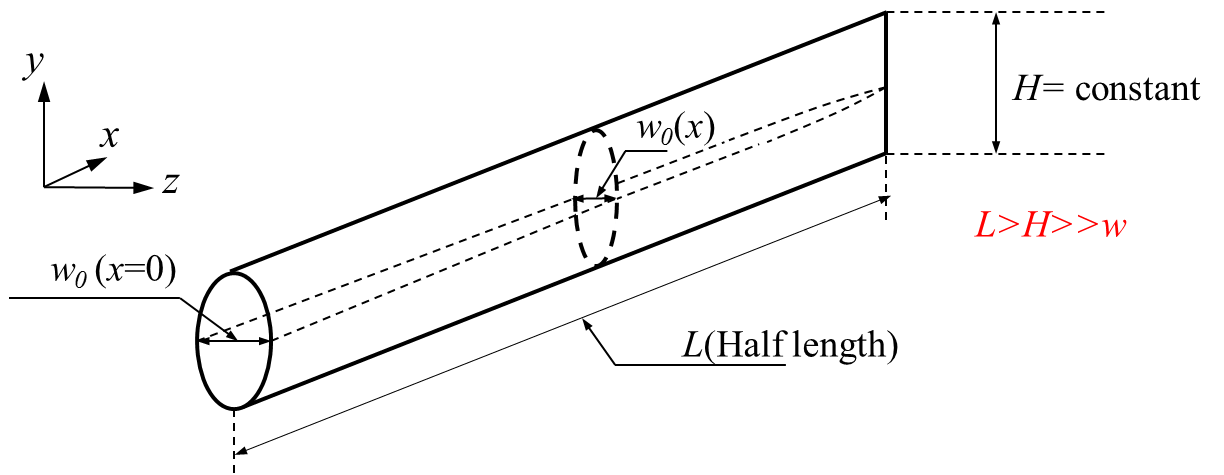
Figure 1: Schematic view of the PKN model (one-wing)
Because the fracture length is large compared to the other two dimensions, the approximate plane strain condition can be assumed in every plane orthogonal to the length (x-axis) [2], which means the net pressure on different vertical planes are not the same as for the exact plane strain condition, but the net pressure is independent of y-axis and the fracture width is calculated from the plane strain solution with this constant pressure on a single vertical plane, making the cross section elliptical [3]:
where: \(w\) and \(p\) are the fracture width and net fluid pressure respectively in a vertical plane and the plane strain Young’s modulus \(E'\) is defined as:
The maximum fracture width at the center of a vertical plane is then given by [3]:
Typically, when the fracture total length (\(2L\)) is more than three times of the height, the error from the plane strain assumption is negligible [4].
The P-K equation
The PKN model was originally raised by Perkins and Kern with the following extra assumptions [5]:
- The formation toughness \(K_{Ic}\) can be neglected because the energy required to propagate in the fracture is significantly less than that required to allow fluid flow along the fracture [4] ;
- The fluid is injected with a constant injection volumetric rate \(Q_0\) from a fixed line source at the center of the fracture into two wings;
- The injected fluid is incompressible Newtonian laminar unidirectional flow characterized with viscosity \(\mu\) and the gravity effect is excluded;
- Constant flow rate \(q\) along the fracture (No storage effect or fluid leakoff);
- The net pressure is zero at the tip.
The fluid continuity equation is [3] :
With the 4th assumption, it can be reduced to:
where: \(q_L\) is the fluid leakoff volume per unit fracture length and \(A\) is the cross-sectional area. The second and third term of Eqn (4) represent the leakoff effect (fluid loss) and storage effect (fracture volume change), respectively.
Then the integration of the basic equation (Eqn (5)) for a Newtonian laminar fluid in an elliptical section yields the very original P-K equation for the bottomhole maximum fracture width \(w_0\) (i.e. \(w_m(x=0)\))in oilfield units (\(Q_0\) in bbl/min, \(w\) in inch, \(E'\) in psi, \(L\) in ft. and \(\mu\) in cp) [5]:
Because the constant flow rate is assumed along the fracture, the volume conservation results in the explicit extended P-K equations for the fracture half length \(L\) ,bottomhole maximum width \(w_0\) and downhole net pressure \(p_0\) (net pressure at \(x=0\))in terms of time \(t\) with S.I. unit [2]:
Note
The P-K equations (Eqn (6) and Eqn (7)) are not consistent with the assumptions made, since \(w_0\) is still dependent on time \(t\), although the dependence is weak when the injection time reaches 2 minutes (its time derivative is about \(10^{-3}\) when \(t>100\)\(\textrm{s}\)). In addition, the neglecting of both storage effect (\(\frac{\partial A}{\partial t}\)) and leakoff effect (\(q_L\)) makes the P-K equations unconvincing if a practical problem includes either effect.
The Nordgren equation
Nordgren improved the P-K equations by removing “the constant flow rate along the fracture” assumption. Consequently, the storage and leakoff effects are considered in the fluid continuity equation as [3]:
The Carter’s equation is assumed applicable for the leakoff term [3]:
where: \(C_L\) is the fluid leakoff coefficient and \(t_0\) is the time at which a specific fracture point gets exposed [3]:
Then the basic equation of fluid flow rate in an elliptical cross-section associated with the above equations yields a non-linear governing PDE [3]:
The derivation of Eqn (11) can be found here.
The non-linear Eqn (11) can only be solved numerically while the analytical approximations can be made in the two following limiting cases by introducing a dimensionless time defined as [3]:
When \(t_D\) <0.01, the problem falls in the small time regime so that no leakoff ( \(q_L\) =0) can be approximated, thus Eqn (11) is reduced to [3]:
(13)\[\frac{E'}{128\mu H}\frac{\partial^2}{\partial x^2}(w_0^4)=\frac{\partial w_0}{\partial t}\]The self-similarity solution is implemented to yield three equations [3]:
(14)\[\begin{split} \begin{equation} \begin{split} L&=0.68\times16^{-\frac{1}{5}}(\frac{Q_0^3E'}{\mu H^4})^{\frac{1}{5}}t^{\frac{4}{5}} \\ w_0&=2.5\times2^{-\frac{1}{5}}(\frac{Q_0^2\mu}{E'H})^{\frac{1}{5}}t^{\frac{1}{5}} \\ p_0&=2.5\times64^{-\frac{1}{5}}(\frac{E'^4Q_0^2\mu}{H^6})^{\frac{1}{5}}t^{\frac{1}{5}} \end{split} \end{equation}\end{split}\]When \(t_D\) >1, the problem falls into the large time regime which is dominated by the fluid leakoff, and the volume change due to the storage effect \(\frac{\partial A}{\partial t}\) is proved to be negligible compared to the leakoff effect in this regime. Thus, the combination of Eqn (8) and Eqn (9) yields:
(15)\[\frac{\partial q}{\partial x}=-\frac{2HC_L}{\sqrt{t-t_0}}\]The solutions to Eqn (15) is obtained by Nordgren as [3] [6]:
(16)\[\begin{split}\begin{equation} \begin{split} L&=\frac{Q_0}{2\pi C_LH}t^{\frac{1}{2}} \\ w_0&=4(\frac{Q_0^2\mu}{\pi^3E'C_LH})^{\frac{1}{4}}t^{\frac{1}{8}} \\ p_0&=2(\frac{E'^3Q_0^2\mu}{\pi^3C_LH^6})^{\frac{1}{4}}t^{\frac{1}{8}} \end{split} \end{equation}\end{split}\]
Note
The Nordgren solution (Eqn (14) and Eqn (16)) is an asymptotic approximations for the PKN model that considers either storage effect or fluid leakoff. The large leakoff solution Eqn (16) is still not consistent with the assumption made because \(w_0\) is still dependent on \(t\). However, this time dependence is weaker than the P-K solution (Eqn (7)) since the power of \(t\) decreases from \(\frac{1}{5}\) (Eqn (7)) to \(\frac{1}{8}\).
Dimensionless analysis
The Nordgren solution (Eqn (14) and Eqn (16)) does not consider the near-tip fracture width \(w\) behavior (the degeneracy of the governing PDE Eqn (11) near the tip due to the vanishing of \(w\)) [7] , and it only considers either storage effect term \(\frac{\partial A}{\partial t}\) or the leakoff term \(q_L\) for the storage-dominated regime and leakoff-dominated regime, respectively. The dimensionless analysis addresses these two issues by exploring the tip asymptotics and adding a perturbation term [8]. Besides, a more accurate \(t_D\) range is determined for the two limiting cases [8]. The dimensionless time \(t_D\) introduced by Nordgren is rewritten as [8]:
where:
Then the two scaling schemes are introduced to the fracture half length and width [8]:
where: \(\bar w\) is the average fracture width defined from the plane-strain condition as Eqn (1): \(\bar w = \frac{H}{\bar E}p\)
The half length scale \(l\), width scale \(W\) and the dimensionless evolution parameter \(P\) take explicit forms for the storage-dominated (m-scaling) regime (small time regime) [8]:
and for the leakoff-dominated(M-scaling) regime (large time regime):
And the variable \(\xi\) is defined as: \(\xi=\frac{x}{L(t)}, (0\le\xi\le1)\).
After scaling the governing equation Eqn (11) with the forms above, the dimensionless fracture half length and width can be obtained by doing the perturbation so that both storage effect and leakoff are considered.
For m-scaling storage-dominated regime [8]:
When \(C_m\) =0 (only the storage effect is considered):
With the perturbation term for correction, the dimensionless fracture half length \(\gamma_m\) can be solved from the analytical equation:
Similarly for the M-scaling leakoff-dominated regime [8]:
When \(S_M\) =0 (only the leakoff is considered):
With perturbation, the dimensionless fracture half length can be solved from the analytical equation:
And there is no analytical expression given for the dimensionless fracture width \(\Omega_m\) and \(\Omega_M\), thus they have to be solved numerically.
In addition, the accuracy \(\varepsilon\) is related to the dimensionless time \(\tau\) by [8]:
Take \(\varepsilon=5\%\), a better dimensionless time range can be determined:
For storage-dominated regime: \(\tau<1.6578\times10^{-5}\);
For leakoff-dominated regime: \(\tau>206.31\);
The the numerical result of the PKN dimensionless fracture half length \(\gamma_f\) can be obtained by:
\(L_f\) is the fracture half length obtained by FrackOptima and \(l\) is introduced as \(l_m\) in Eqn (18) or \(l_M\) Eqn (19).
Then comparisons can be made with the analytical \(\gamma\) and the difference is defined as:
Note
The dimensionless analysis results are the improved approximations for the PKN model that considers the neat-tip fracture width behavior and correct Nordgren’s solution, which only considers either storage or leakoff, by adding a perturbation term with the first-order analysis.
FrackOptima result
The storage-dominated case
Example 1(moderate viscosity):
All the examples for a moderate viscosity are set with fracture height \(H=20 \textrm{m}\)
- Young’s modulus \(E =30(\textrm{GPa})\)
- Poisson ratio \(\nu =0.2\)
- Rock toughness \(K_{Ic} =1.1(\textrm{MPa} \bullet \sqrt{\textrm{m}})\)
- Leakoff coefficient \(C_L =0( \textrm{m/}\sqrt{\textrm{sec}})\)
- Fluid viscosity \(\mu =0.05(\textrm{Pa}\bullet \textrm{sec})\),
- Pumping rate \(Q_0 =0.1(\textrm{m}^3/\textrm{sec})\)
- Pumping time \(t =900(\textrm{sec})\),
Thus, \(\tau =0<\tau_{storage}=1.6578\times10^{-5}\)
This example will be presented in details to illustrate how to make appropriate inputs so that a numerical result can be obtained for comparison.
Material Database
Firstly the fluid parameters are entered in the Fluids subpanel of the Material Database panel, as shown in Figure 2. Because the fluid is assumed to behave as a Newtonian laminar flow so that the Behavior Index value should be \(\textrm{1}\). Also, we set both Has Crosslinker and Has Breaker are False so that the fluid viscosity remains constant. In addition, a zero density is specified since the fluid density is not considered in PKN model. However, if a non-zero density is input, a constant stress profile has to be specified in the Layer Stress subpanel of the Reservoir Formation to overcome it [9].
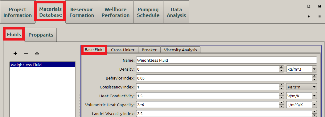
Figure 2: Input the fluid parameters
The proppant parameters are specified as shown in Figure 3, although it is not involved in the PKN model. If the proppant is not specified here, the Pumping Schedule panel yields an error indicator as shown later in the blue box in the Figure 10.
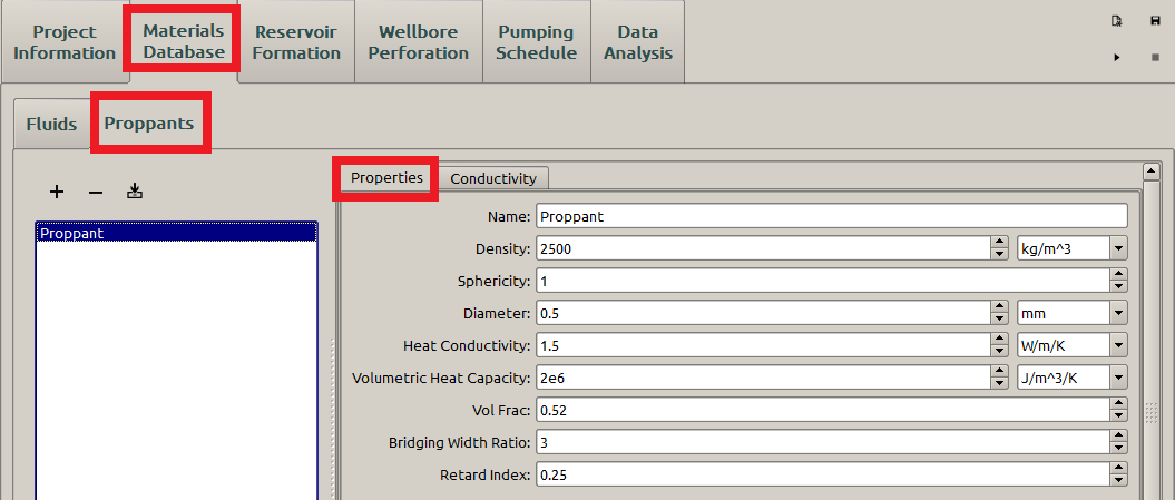
Figure 3: Input the proppant parameters
Reservoir Formation
Then the formation properties need specifying , the PKN model assumes homogeneous and isotropic formation, thus the input of the Reservoir Formation here is very similar to the one of KGD. The Interface input is displayed in Figure 4. Here, the fracture height is chosen as \(\textrm{20 m}\) and the fracture half length can be approximated with Eqn (14) as about \(\textrm{470 m}\). Thus, we may choose \(\textrm{2.5 m}\) for the element size across the layer and \(\textrm{5 m}\) for the one along the layer, since \(8\) vertical elements is reasonable for the numerical computation and meanwhile a reasonable size ratio should be kept for the element (\(1:2\) here).
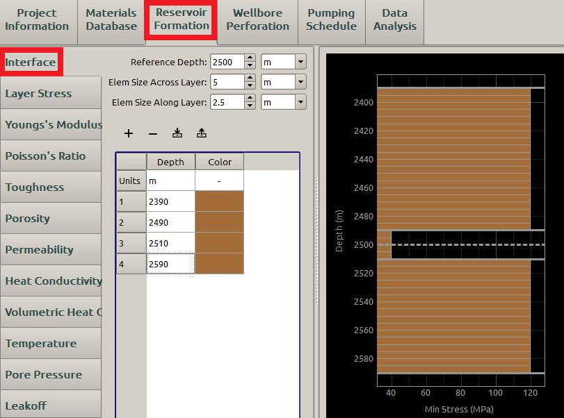
Figure 4: Input the interface parameters
Then, the Stress input is shown in Figure 5. Please notice that the same Depth cannot bear different stress values, thus the stress interface should be set up by evaluating two different stresses to two nearby depths. For example, the depth \(\textrm{2490 m}\) is a single interface so that one set of stresses is evaluated to \(\textrm{2490 m}\) and the other set is evaluated to the near one \(\textrm{2489.99 m}\).
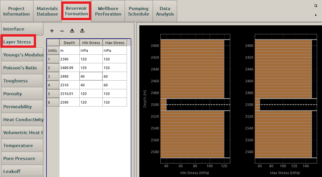
Figure 5: Input the stress parameters
The uniform formation toughness input is displayed Figure 6. The considerably large stress difference is set up here to ensure the well confinement of the fracture height, while the toughness is uniform so that the numerical simulation is closer to the PKN model.
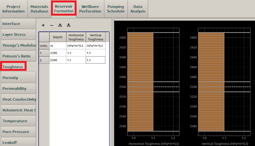
Figure 6: Input the stress parameters
Other relevant formation parameters are Young’s modulus, Poisson ratio and leakoff coefficient. Other formation parameters does not need specifying for the PKN model. An example of the leakoff coefficient input is shown in Figure 7.
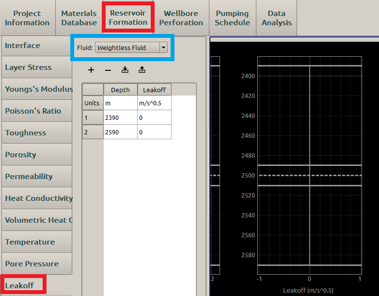
Figure 7: Input the leakoff coefficient
Wellbore Perforation
Having specified the material and formation parameters, we can begin to define the wellbore and perforation parameters in Wellbore Perforation panel. First the wellbore can be specified in Wells subpanel as shown in Figure 8.
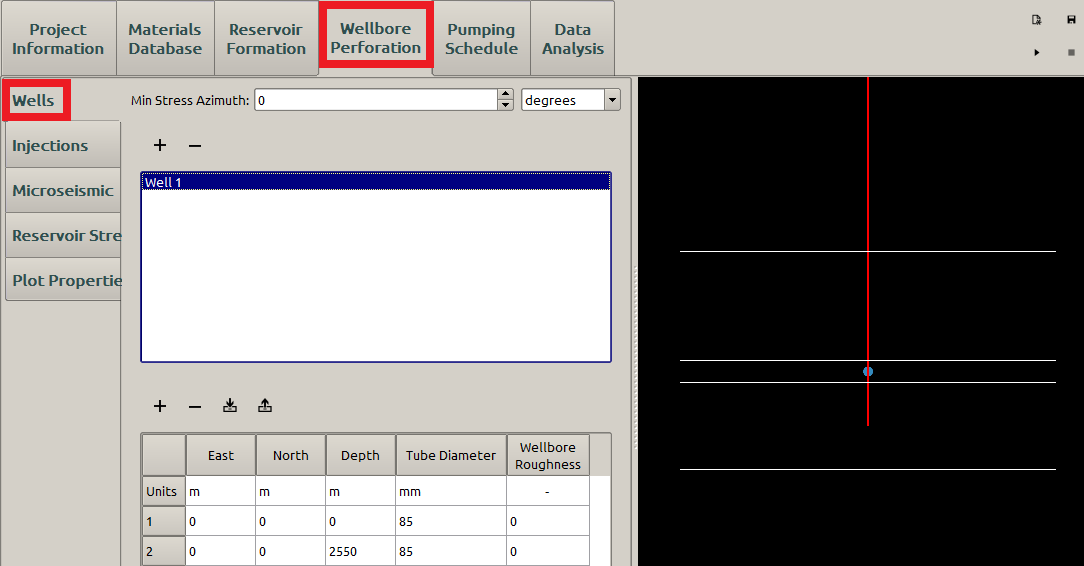
Figure 8: Input the wellbore location parameters
In hydraulic fracturing, the fracture is assumed to open in the direction of the horizontal minimum stress \(\sigma_\textrm{h,min}\). Thus, the PKN model opens in horizontal planes, forming a vertical planar long fracture consequently as shown in Figure 11. Therefore, the horizontal minimum stress azimuth \(\alpha\) will not affect the fracture propagation in PKN model. Then we put \(0\) for the MinStress Azimuth. In addition, Neither the wellbore friction nor the perforation erosion is not considered here, so the Wellbore Roughness and Perforation Erosion Coefficient are both \(0\).
The injection location can be specified in Injections subpanel as shown in Figure 9. Here only one injection is specified because it is convenient to read the net pressure at the bottomhole directly after the simulation, otherwise the net pressure is calculated for each injection and we have to use the downhole pressure to calculate the bottomhole net pressure. In addition, \(50\) Number of Perforations are used to ensure a negligible perforation pressure drop if non-zero density is specified in Material Database.
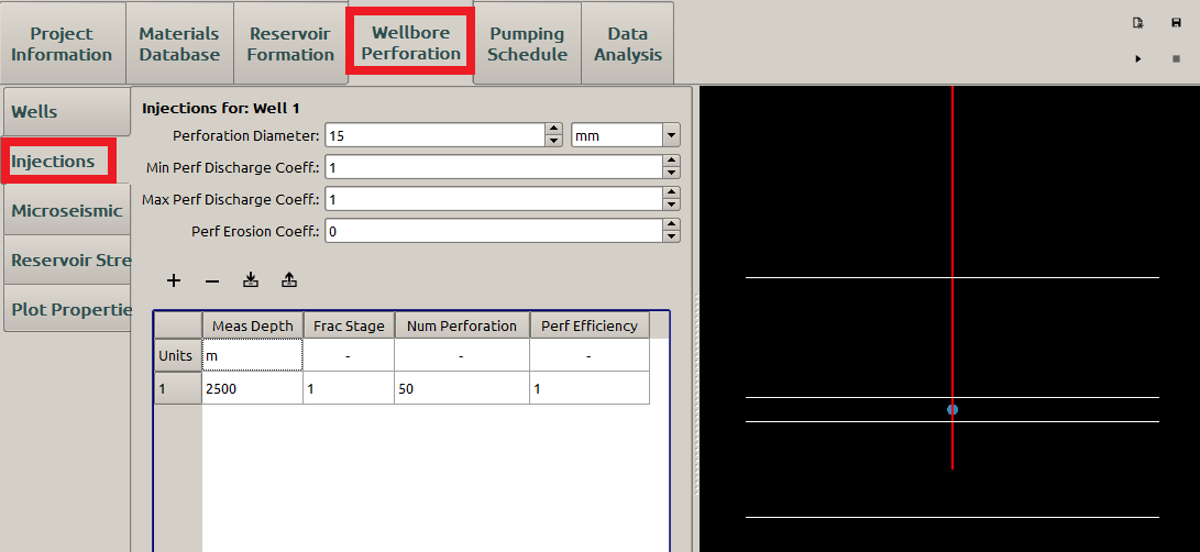
Figure 9: Input the injection location parameters
The Perforation Erosion Coefficient is set zero to exclude the perforation pressure drop.
Pumping Schedule
The inputs of the Pumping Schedule panel may be specified as shown in Figure 10. The proppant menu marked in the green rectangular must be specified with the one defined as in Figure 3 otherwise a red error indicator appears. The parameters associated with proppant are all set to zero because it is not involved within the PKN model.
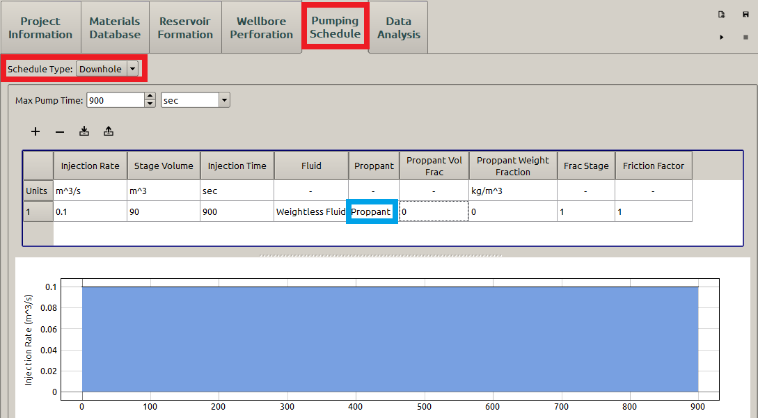
Figure 10: Input the pumping schedule
Similar to KGD examples, neither Microseismic Data nor Reservoir Stress panel is involved for PKN model. Thus they are not taken into account for the theoretic PKN model.
The 3D PKN fracture is as shown in Figure 11.
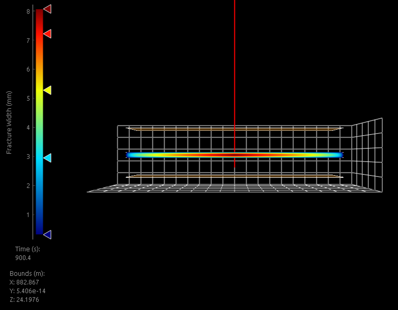
Figure 11: 3D PKN fracture width
Because only one injection is specified in Injection Locations (Figure 9), thus the net pressure can be directly read from the simulator (Figure 12).
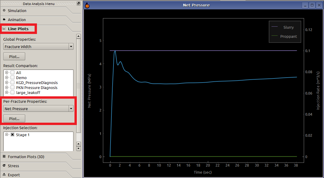
Figure 12: PKN net pressure data for single injection location
If multiple injection locations are specified, the net pressure can not be directly read from the simulator (3 injections in Figure 13). Then, we have to calculate it through the downhole pressure (downhole pressure minus the minimum formation stress).
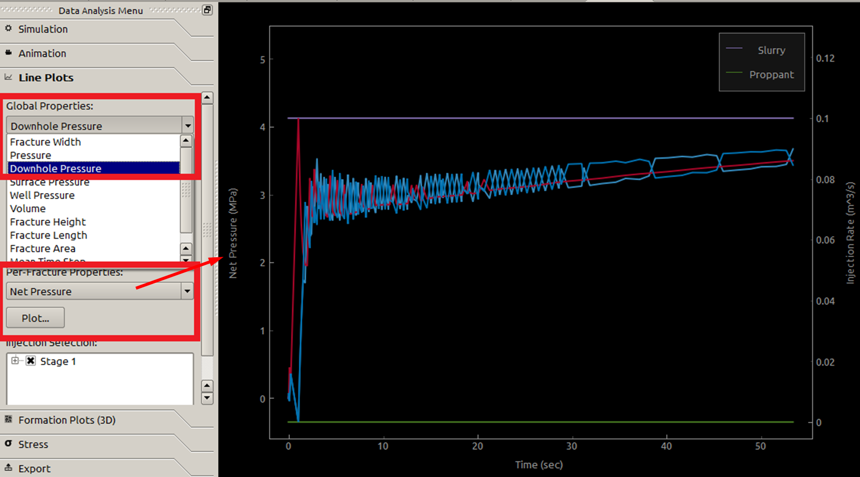
Figure 13: PKN net pressure data for multiple injection locations
Having input all the parameters, we can start the simulation and get the result for the storage-dominated regime as shown in Table 1.
Example 2(low viscosity):
All the examples for a moderate viscosity are set with fracture height \(H=40 \textrm{m}\)
- Young’s modulus \(E =60(\textrm{GPa})\)
- Poisson ratio \(\nu =0.2\)
- Rock toughness \(K_{Ic} =1.1(\textrm{MPa} \bullet \sqrt{\textrm{m}})\)
- Leakoff coefficient \(C_L =0(\textrm{m/}\sqrt{\textrm{sec}})\)
- Fluid viscosity \(\mu =0.001(\textrm{Pa}\bullet \textrm{sec})\),
- Pumping rate \(Q_0 =0.24(\textrm{m}^3/\textrm{sec})\)
- Pumping time \(t =450(\textrm{sec})\)
- Element size \(5\times10(\textrm{m})\).
Thus, \(\tau =0<\tau_{storage}=1.6578\times10^{-5}\)
Result comparison
| Example 1 | Example 2 | |
|---|---|---|
| \(L/H\) | \(21.03\) | \(15.22\) |
| Dimensionless time \(\tau\) | \(0.0\) | \(0.0\) |
| Analytical \(\gamma\) | \(0.6304\) | \(0.6604\) |
| FrackOptima \(\gamma_f\) | \(0.6264\) | \(0.6232\) |
| Difference \(\%\) | \(-5.15\) | \(-5.63\) |
Note
- The rock toughness here (\(K_{Ic} =1.1(\textrm{MPa} \bullet\sqrt{\textrm{m}})\) is relatively large. The results are expected to be more accurate if a smaller toughness value, e.g. (\(K_{Ic} =0.5(\textrm{MPa} \bullet\sqrt{\textrm{m}})\)), is chosen, since the PKN model assumes neglected toughness.
- The Nordgren solution and the dimensionless solution to PKN model is based on a number of assumptions of simplified fracture configuration, for example an elliptical profile across the height. Strictly speaking, what is simulating here by FrackOptima is not exactly an PKN model but should approach it if the \(\textrm{L/H}\) is significantly large enough. Thus, \(\textrm{L/H}>10\) is always kept for the PKN comparison here.
The leakoff-dominated case
Example 3:
- Young’s modulus \(E =30(\textrm{GPa})\)
- Poisson ratio \(\nu =0.2\)
- Rock toughness \(K_{Ic} =1.1(\textrm{MPa} \bullet \sqrt{\textrm{m}})\)
- Leakoff coefficient \(C_L =3.54\times10^{-4}(\textrm{m/}\sqrt{\textrm{sec}})\)
- Fluid viscosity \(\mu =0.05(\textrm{Pa}\bullet \textrm{sec})\),
- Pumping rate \(Q_0 =0.12(\textrm{m}^3/\textrm{sec})\)
- Pumping time \(t =8100(\textrm{sec})\),
- Fracture height \(H =20(\textrm{m})\),
- Element size \(2.5\times5(\textrm{m})\).
Thus, \(\tau =375.5>\tau_{leakoff}=206.31\)
Example 4:
- Young’s modulus \(E =60(\textrm{GPa})\)
- Poisson ratio \(\nu =0.2\)
- Rock toughness \(K_{Ic} =1.1(\textrm{MPa} \bullet \sqrt{\textrm{m}})\)
- Leakoff coefficient \(C_L =1.65\times10^{-4}(\textrm{m/}\sqrt{\textrm{sec}})\)
- Fluid viscosity \(\mu =0.001(\textrm{Pa}\bullet \textrm{sec})\),
- Pumping rate \(Q_0 =0.24(\textrm{m}^3/\textrm{sec})\)
- Pumping time \(t =6300(\textrm{sec})\),
- Fracture height \(H =40(\textrm{m})\),
- Element size \(5\times10(\textrm{m})\).
Thus, \(\tau =310.78>\tau_{leakoff}=206.31\)
The results for leakoff-dominated regime are as shown in Table 2.
Result comparison
| Example 3 | Example 4 | |
|---|---|---|
| \(L/H\) | \(11.49\) | \(10.91\) |
| Dimensionless time \(\tau\) | \(375.5\) | \(310.78\) |
| Analytical \(\gamma\) | \(0.3059\) | \(0.3050\) |
| FrackOptima \(\gamma_f\) | \(0.3041\) | \(0.3023\) |
| Difference \(\%\) | \(-0.59\) | \(-0.89\) |
The comparisons indicate that FrackOptima simulator yields good results that match the theoretical ones well.
| [1] | Yew: Mechanics of Hydraulic Fracturing. Gulf Publishing Company,Houston,USA (1997) |
| [2] | (1, 2) Valko, Economides: Hydraulic Fracture Mechanics. Wiley,Chichester, UK (1995) |
| [3] | (1, 2, 3, 4, 5, 6, 7, 8, 9, 10, 11) Nordgren: Propagation of vertical hydraulic fractures. JPT 253,306-314 (1972) |
| [4] | (1, 2) Economides, etc.: Reservoir Stimulation. 3rd edn. Wiley, Chichester,UK (2000) |
| [5] | (1, 2) Perkins, Kern: Widths of hydraulic fractures. JPTT 222,937-949 (1961) |
| [6] | Geertsma, de Clerk: A Rapid Method of Predicting Width and Extent of Hydraulically Induced Fractures. JPT 246, 1571-1581 (1969) |
| [7] | Kemp: Study of Nordgren’s equation of hydraulic fracturing, SPE Production Eng. 5, 311-314 (1990) |
| [8] | (1, 2, 3, 4, 5, 6, 7, 8) Kovalyshen, Detournay: A Reexamination of the Classical PKN Model of Hydraulic Fracture, TPM. 81, 317-339 (2010) |
| [9] | Zhai, Fonseca, Azad and Cox: A new tool for multi & multi-well hydraulic fracture modeling, SPE-173367-MS (2015) |