Project¶

The Project tab is where you can manage projects and specify miscellaneous information about the current project. Projects can be created from the Project List on the left side of the software window (larger red box in Figure 1). Above the Project List is the Working Directory selector (blue box in Figure 1).

Project List¶

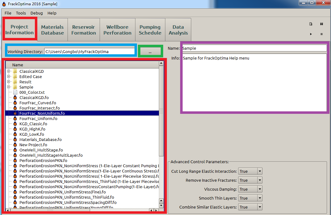
Figure 1: Project tab

On the left side of the software window is the Project List, which displays all the files in the current working directory. This is where a user can Load, Rename a project, or Open in file explorer. Right-clicking a project file brings up a context menu with which to perform these actions (Figure 2).

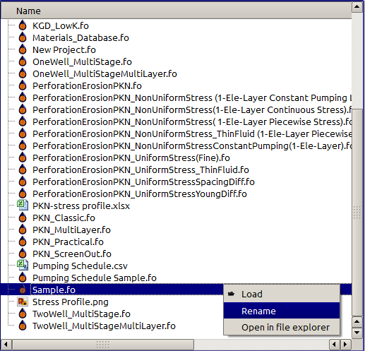
Figure 2: Project actions

Action	With project selected	No selection
Load	Load selected project	Nothing
Rename	Rename selected project	Nothing
Open in file explorer	Open the folder containing the selected file	Nothing

Working Directory¶

The current Working Directory is shown above the Project List (blue box in Figure 1). The working directory is where all of the information about projects, results, and the materials database are stored.

To change the working directory, simply click the button to the right of the current working directory text. A dialog will pop up asking for the location of the new working directory (green box in Figure 1).

To the left of the working directory, thu user can directly rename the project and enter some information about the project in the “Name” and “Info” (purple box in Figure 1), respectively.

Advanced Control Parameters¶

All the advanced control parameters listed here(Figure 3), if chosen True, are applied for a more efficient(faster) simulation. Because the True options add more approximations on the simulation, leading to a higher computation speed.

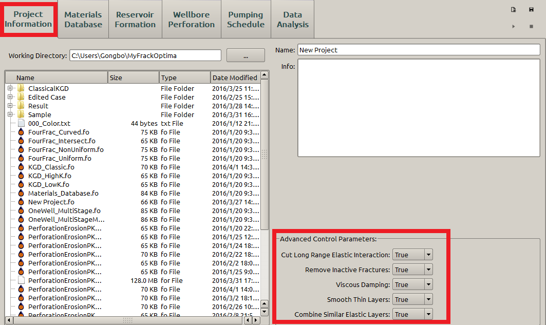
../_images/advanced-control-parameter.png

Figure 3: Advanced control parameters

Cut Long Range Elastic Interaction¶

According to the displacement discontinuity method (DDM), which is implemented in FrackOptima to model the elastic interaction, the stress $\sigma_{ij}$ between two elements (i.e. the stress at the $i\textrm{th}$ element due to the displacement discontinuity at the $j\textrm{th}$ element) is inversely proportional to the square of the distance of these two elements $r_{ij}$ (Figure 4).

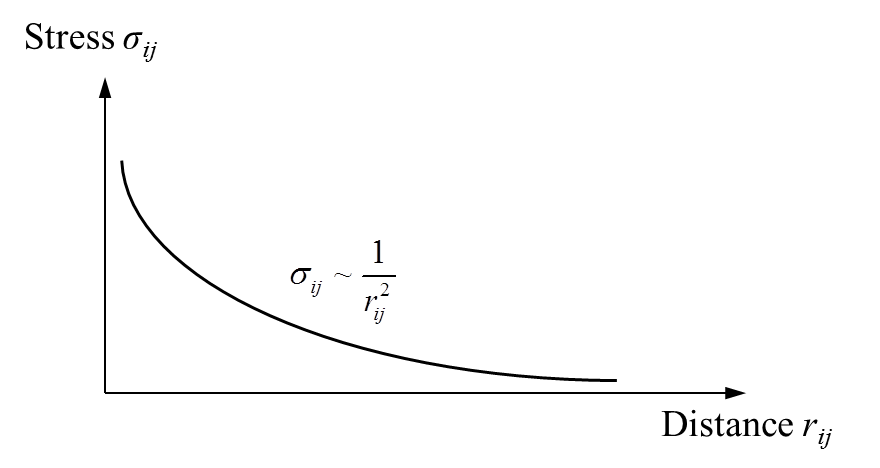
Figure 4: Stress vs. Distance in DDM (schematic view)

Thus, when $r_{ij}$ is large enough, the elastic interaction of these two elements ($\sigma_{ij}$) becomes insignificant. FrackOptima treats $\sigma_{ij}=0$, when $r_{ij} \geq 10.5\textrm{e}_\textrm{h}$, where $\textrm{e}_\textrm{h}$ represents the element size along the layer, if Cut Long Range Elastic Interaction is set True. When it is set False, the $\sigma_{ij}$ will be calculated according to DDM, no matter how far away two elements space.

Remove Inactive Fractures¶

During a hydraulic fracturing treatment, the fluid in one or some fractures may all leaked off (the blank fracture at the left side in Figure 5).

$../_images/empty-fracture.png$

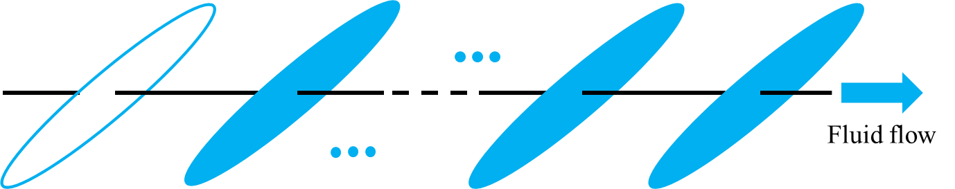
Figure 5: An inactive fracture in the treatment (schematic view)

With the inside fluid being all leaked off, there are only proppants remaining in the fracture, leading to a fracture width, denoted by $\textrm{w}_0$, which does not change with time. Let us denote the fracture width of other fractures containing fluids by $\textrm{w}_1$. The elastic interaction equation can be written as:

(1)\[\begin{split}\left[ \begin{array}{ccc} \textrm{K}_{00} & \textrm{K}_{01} \\ \textrm{K}_{10} & \textrm{K}_{11} \\ \end{array} \right] \left[ \begin{array}{ccc} \textrm{w}_0 \\ \textrm{w}_1 \\ \end{array} \right] = \left[ \begin{array}{ccc} \textrm{p}_0 \\ \textrm{p}_1 \\ \end{array} \right]\end{split}\]

where:

$\textrm{K}$ represents the elastic interaction matrix obtained from the displacement discontinuity method (DDM), $\textrm{w}$ is the fracture width, and $\textrm{p}$ is the pressure inside fractures.
The subscript $0$ and $1$ represent the parameters associated with inactive fracture (without fluid inside) and active fracture (with fluid inside), respectively.

If Remove Inactive Fractures is set False, the simulation solves the whole Eqn (1). Otherwise, Eqn (1) is decomposed to:

(2)\[\textrm{K}_{10}\textrm{w}_0 + \textrm{K}_{11}\textrm{w}_1 = \textrm{p}_1\]

Eqn (2) is the part pertaining only to time-dependent variables of Eqn (1). In other words, the simulation only solves the time-dependent part of (1), leading to a smaller size of system equations and, as a result, a more efficient computation.

If the inactive fracture is far from ($r \geq 10.5\textrm{e}_\textrm{h}$) some active fractures (for example the inactive fracture and the most right side active fracture in Figure 5), the Cut Long Range Elastic Interaction may be also set True to yield a even more efficient simulation.

Note

Even with the Remove Inactive Fractures as True, only a completely fluid-depleting fracture (all the elements of the fracture has zero fluid volume) can be treated as inactive. Any partially fluid-depleting fractures (not all the elements of a fracture has zero fluid volume) are still active.

Viscous Damping¶

To maintain the numerical stability, a sufficiently small time step $\triangle t$ is required for the hydraulic fracturing simulation. $\triangle t$ is proportional to the fluid viscosity $\mu$ and inversely proportional to the cubic of fracture width $\textrm{w}$:

(3)\[\triangle t \sim \mu \bigg( \frac{\textrm{e}}{\textrm{w}} \bigg)^3\]

where, $\textrm{e}$ represents the element size.

Thus, when a thin fluid (fluid with low viscosity, for example slickwater) flows through a relative wide but short fracture, i.e. small $\big( \frac{\textrm{e}}{\textrm{w}} \big)^3$ value, $\triangle t$ could be prohibitively small, leading to an extremely slow simulation. The Viscous Damping is then introduced in FrackOptima to overcome this issue. When $\triangle t$ is less than a criteria, for example $\log_{10} \triangle t \leq -3$, the viscosity $\mu$ will be increased artificially to a value that compensates the small $\big( \frac{\textrm{e}}{\textrm{w}} \big)^3$ value to maintain a reasonable $\triangle t$, while the accuracy of the whole simulation will not be sacrificed significantly.

Smooth Thin Layers¶

In a numerical simulation, the element size $\textrm{e}$ cannot be too large resulting to numerical inaccuracy; meanwhile according to Eqn (3) it cannot be too small either in order to maintain a reasonable time step. Thus, the value of $\textrm{e}$ for a simulation usually falls in some range.

When the reservoir formation for a hydraulic fracturing treatment is a multi-layered media (Figure 6), the thickness of an individual layer $\textrm{d}$ cannot be too small compared to the element size $\textrm{e}$, otherwise the numerical stability will be deteriorated. In FrackOptima, it is preferable that $\textrm{d}\geq 0.75\textrm{e}$.

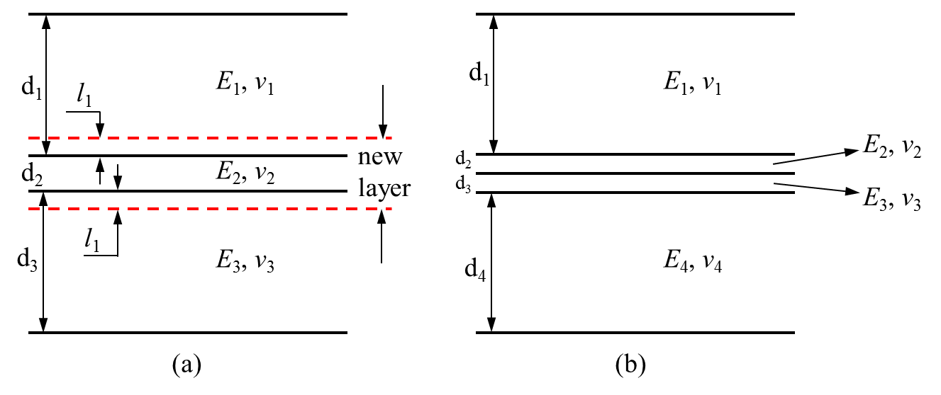
Figure 6: Thin layer(s) in a multi-layered media (schematic view)

There are two situations to apply Smooth Thin Layers:

A single thin layer with $\textrm{d}< 0.75\textrm{e}$ is sandwiched by thick layers ( the second layer in Figure 6 (a)). Then the original thin layer will be mixed with part of the adjacent layers such that the new layer thickness falls in the range $[0.75\textrm{e}, 1.5\textrm{e}]$ by following the rule of mixture:

(4)\[\bar A = \frac{\sum_{i=1}^{n}A_id_i}{\sum_{i=1}^{n}d_i}\]

where:

$A$ represents the reservoir formation properties of an individual layer, for example, Young’s modulus and Poisson’s ratio, etc. The $\bar A$ represents the effective reservoir formation properties of the new layer.
$n$ is the total number of thin layers, including the part of thick layers, which are going to be smoothed. $d_i$ is the thickness of these thin layers. For example, there are totally $3$ layers that are going to be smoothed (the second layer, and the part of the first and third layer) in Figure 6 (a).

The other smooth situation is for the multiple thin layers, as illustrated in Figure 6 (b). If the new layer generated by smoothing all the original thin layers with the rule of mixture (Eqn (4)) is thicker than $0.75\textrm{e}$, no more smooth is needed then. On a contrary, if the new layer is still thinner than $0.75\textrm{e}$, then the procedure in the first situation is going to be applied.

Note

If the Smooth Thin Layers is set as False, a yellow warning indicator and a warning pop-up will be displayed (Figure 7). Because the False option may result in numerical instability when $\textrm{d}<0.75\textrm{e}$.

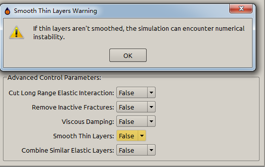
Figure 7: Thin layer warning indicator

Combine Similar Elastic Layers¶

If the Young’s modulus and Poisson’s ratio in adjacent layers are within $10\%$ difference, they can get combined as a uniform layer to accelerate the simulation. An example is given as in Figure 8.

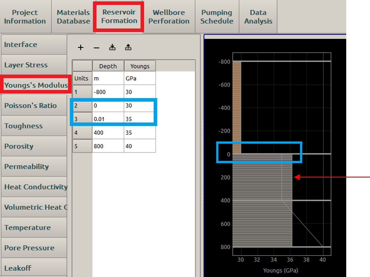
../_images/youngs-modulus-input-combined.png

Figure 8: Combined Young’s modulus

In Figure 8, there are three user-defined layers ( $-800\textrm{m}$ to $0\textrm{m}$, $0\textrm{m}$ to $400\textrm{m}$, and $400\textrm{m}$ to $800\textrm{m}$), all of which are assumed of the same Poisson ratio. According to the user’s inputs, the first two layers are of uniform Young’s modulus as $E_1=30\textrm{GPa}$ and $E_2=35\textrm{GPa}$. These two values differ more than $10\%$, thus they are not going to be combined. In each user-defined layer, the Young’s modulus and Poisson’s ratio are set as uniform by FrackOptima. Thus, the third layer with a linear increasing Young’s modulus ( $E$ from $35$ to $40\textrm{GPa}$) is interpreted as with the uniform $E_3=37.5\textrm{GPa}$. Then, $E_2$ differs from $E_3$ less than $10\%$, these two layers get combined as one new layer with $E_4=36.25\textrm{GPa}$ (pointed by the red arrow) when Combine Similar Elastic Layers is True. The grey straight vertical line with value $35\textrm{GPa}$ connecting a downward slope ending with $40\textrm{GPa}$ represents the user’s original inputs.

When Combine Similar Elastic Layers is False, the layers are not going to be combined, as illustrated in Figure 9. The Young’s modulus of the three layers are: $E_1=30\textrm{GPa}$, $E_2=35\textrm{GPa}$, and $E_3=37.5\textrm{GPa}$.

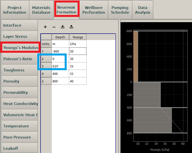
../_images/youngs-modulus-input-no-combination.png

Figure 9: Young’s modulus without combination