Materials Database
Introduction
The Materials Database panel is where a user can specify a set of fluids and proppants to be used in other parts of FrackOptima. Under each of the two subpanels (Fluids and Proppants), three buttons (Figure 1) are available for the users to add, delete or import fluids/proppants.
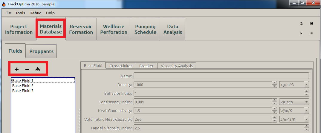
Figure 1: Three buttons
See also
- Importing and Exporting
- For more information on importing and exporting in general.
- Tables
- For more information on tables in FrackOptima.
Form View
The materials under Material Database are displayed in the Form View, where the material properties is edited as a form. In particular, the Fluids form view is shown in Figure 2.
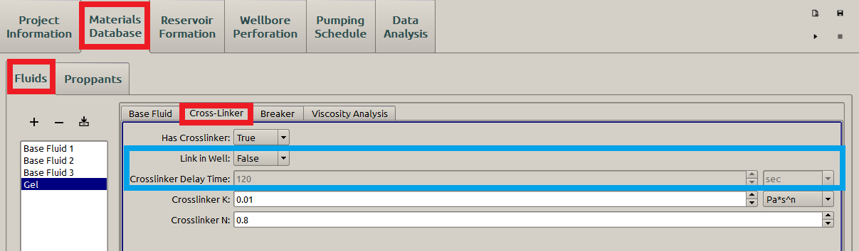
Figure 2: Form view for fluids
Figure 2 shows properties of the cross-linker based on the Base Fluid. The parameters in this subpanel will be explained in the following sections.
Note
Whenever selecting a material from a drop down menu in another part of FrackOptima, the currently highlighted material’s properties will by shown in a tooltip. For example, in Figure 3 the Gel’s property is displayed in a tooltip under the Pumping Schedule panel.
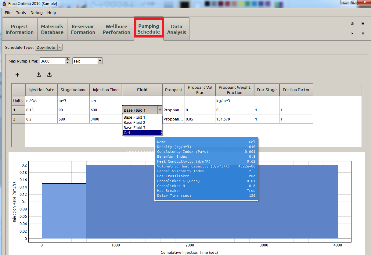
Figure 3: Gel’s property displayed in Pumping Schedule
Fluids
Fracking fluids used in the pumping schedule are defined in the Fluids subpanel. The particles made of solid materials and contained in fracking fluids, known as the proppants, are going to be defined in the Proppants subpanel.
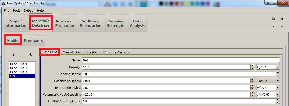
Name
The name input gives a name to a fluid which will be used in the Pumping Schedule panel. Different fluids should have different names.
Density
The density of a substance, denoted by \(\rho\), is its mass per unit volume. It can be mathematically defined by the equation:
where: \(m\) and \(V\) are the mass and volume of the substance, respectively, so that the S.I. unit of density is \(\textrm{kg/m}^3\)
In some classical hydraulic fracturing models, e.g. PKN and KGD, the fluid weight is excluded from consideration. In such conditions, the density can be set as \(0\) .
Behavior Index and Consistency Index
For some incompressible steady-state fluids in 1D laminar flow, the shear stress \(\tau\) is linearly related to the local shear rate as in Eq. (2) , which is known as the Newton’s law, and illustrated in the Figure 4 [1] :
where:
- \(u\) is the unidirectional velocity of the upper plate, \(\textrm{m/s}\)
- \(\dot{\gamma}\) is the shear rate, \(\mathrm{s}^{-1}\)
Fluid that is characterized by Newton’s law (Eq. (2) ), with the proportionality \(\mu\) independent of the shear rate, is called Newtonian fluid. For a newtonian fluid, \(\mu\) is the fluid viscosity, with SI units \(\textrm{Pa} \bullet \textrm{s}\). Viscosity is a measure of the fluid’s resistance to gradual deformation by shear stress.

Figure 4: Schematic representation of a unidirectional shearing flow between two parallel plates
Fluid that does not behave according to Newton’s law is non-Newtonian fluid, which may be characterized by the power-law equation:
where:
- \(\textrm{n}\) is the behavior index, dimensionless
- \(\textrm{K}\) is the consistency index, and is analogous to viscosity in Newton’s law, \(\textrm{Pa} \bullet \textrm{s}^n\)
Fluids that behave according to Eq. (3) are called power-law fluids. FrackOptima treats the non-Newtonian fluids as power-law fluids. When the behavior index \(\textrm{n=1}\), the power-law fluid is reduced to the Newtonian fluid and the consistency index \(\textrm{K}\) equals the fluid viscosity \(\mu\).
At room temperature (about \(\textrm{300 K}\)), water can be treated as a Newtonian fluid. Thus, the behavior index is \(1\) and the consistency index (viscosity) can be taken as \(\mathrm{0.001 Pa} \bullet \mathrm{s}\), which may also be used for slickwater in hydraulic fracturing.
Heat Conductivity
Heat Conductivity, also known as thermal conductivity, characterizes a material’s ability to conduct heat when subjected to temperature gradient. It is the proportionality constant, denoted as \(\lambda\), in Fourier’s law for heat conduction, shown in Eq. (4) :
where:
- \(\varphi\) is the heat flux, \(\textrm{W}/\textrm{m}^2\)
- \(\nabla T\) is the temperature gradient, \(\textrm{K/m}\)
- The minus sign “-” means the heat flux always flows from the warmer area (higher temperature) to the colder one (lower temperature).
The heat conductivity of non-metals may be assumed to be constant in the temperature range in hydraulic fracturing [2]. At room temperature (about \(\textrm{300 K}\)), the heat conductivity of liquid water is \(\textrm{0.58 W}/(\textrm{m} \bullet \textrm{K})\) [3], which may be used for slickwater in hydraulic fracturing.
Volumetric Heat Capacity
Volumetric heat capacity, usually denoted as \(c_v\), characterizes the ability of a given volume of a substance to store internal energy while undergoing a given temperature change, but without undergoing a phase change.
At room temperature (about \(\textrm{300 K}\)), the volumetric heat capacity of liquid water is \(\textrm{4.18 MJ}/(\textrm{K} \bullet \textrm{m}^3)\) [4], which may be used for slickwater in hydraulic fracturing.
Landel Viscosity Index
Fracturing fluid generally contains solid particles, called proppants to keep hydraulically-induced fractures open after the pumping. Thus, the concentration of proppants affects the viscosity of the fluid-proppant mixture, also known as a slurry. A number of expressions are developed to determine the viscosity of slurries. A well-accepted one is the Landel equation [5] [6]:
where:
- \(\mu\) is the viscosity of the fluid with particles
- \(\mu_0\) is the viscosity of the clean fluid
- \(c\) is the volume fraction of particles
- \(c_{max}\) is the maximum volumetric particle concentration
- \(\textrm{m}\) is the Landel viscosity index, a typical value of \(\textrm{m}\) is 2.5
Viscosity Temperature Decay, Has Crosslinker, Has Breaker and other Fluid Rheology Parameters
Apparent Viscosity
Eq. (3) can be rewritten in a form similar to Newton’s law:
where:
- \(\mu_a\) is the apparent viscosity, and is analogous to Newtonian fluid viscosity, \(\textrm{Pa} \bullet \textrm{s}\)
- \(\textrm{K}\) is the consistency index
- \(\textrm{n}\) is the behavior index
- \(\dot{\gamma}\) is the shear rate
This simple relationship approximates Newtonian behavior of the behavior index \(n \approx 1\), in which case the consistency index \(\textrm{K} \approx\mu_{a}\). A shear-thinning fluid, which is common in hydraulic fracturing, is one in which \(\textrm{n} < 1\). The apparent viscosity of a shear-thinning fluid decreases as the velocity gradient of the fluid increases. Analogously, a shear-thickening fluid has \(\textrm{n} > 1\), and its apparent viscosity increases as the velocity gradient increases.
The fracturing fluid in FrackOptima is modeled as a mixture containing base fluid (including polymer), crosslinker, breaker and proppant pack (Figure 6). The apparent viscosity \(\mu_a\) of this mixture is a function of time, temperature and proppant concentration theoretically. However, the temperature-dependence of \(\mu_a\) is insignificant compared to the time-dependence one due to the breakers. Thus, FrackOptima simplifies the complexity of \(\mu_a\) by neglecting the temperature-dependence.
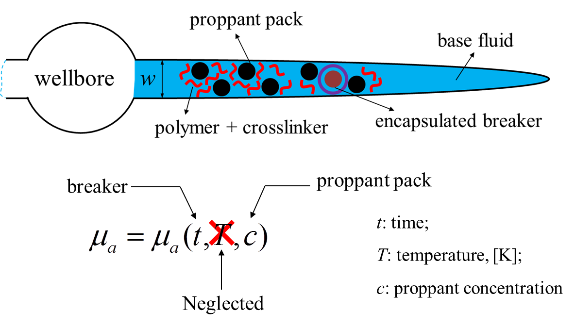
Figure 6: Fracturing fluid components and the dependencies of its apparent viscosity
Overall speaking, \(\mu_a\) is desired to be relatively low in the wellbore to reduce the friction pressure (see Figure 7), sufficiently high in the hydraulic fractures for a better proppant transportation, and low again after pumping, when the fractures are obtained, for an easier removal of the remaining fluid to facilitate hydrocarbons production.
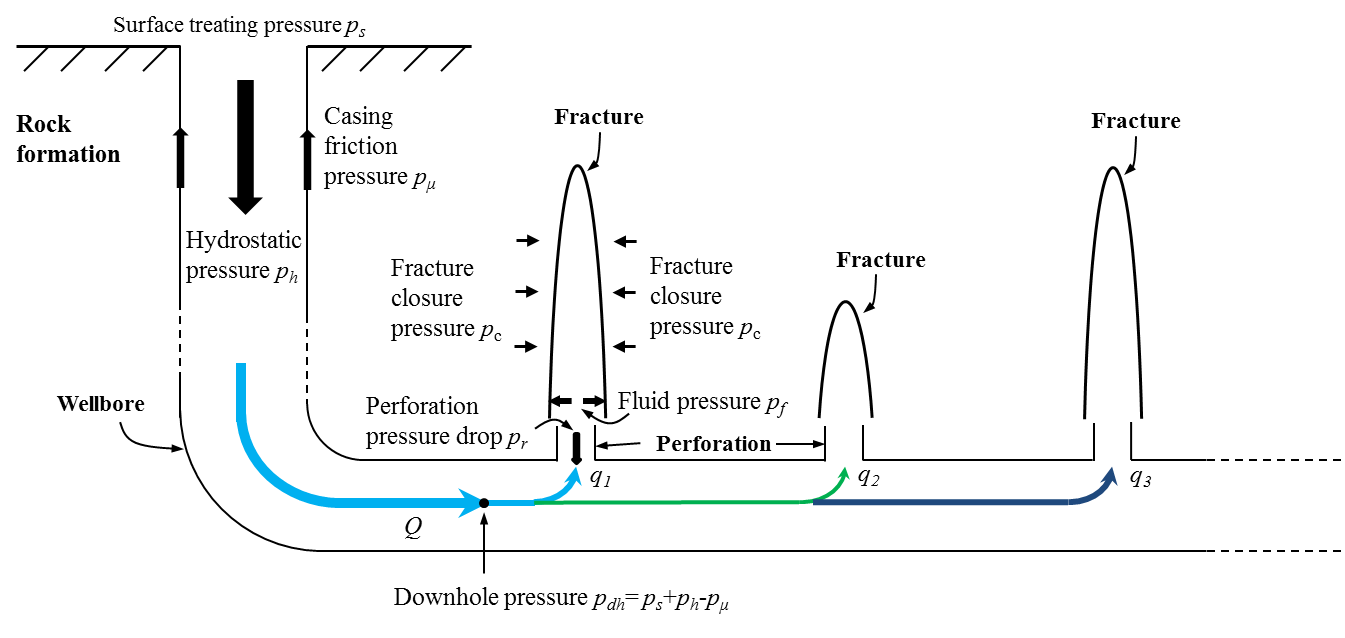
Figure 7: Schematic view of the pressure distribution in a wellbore
FrackOptima models \(\mu_a\) with the following equations:
where:
\(\mu_{a0}\) is the apparent viscosity of the base fluid (Figure 5), \(\textrm{Pa} \bullet \textrm{s}\)
\(\textrm{K}\) and \(\textrm{n}\) are the consistency index and the behavior index of the base fluid. Both of them are functions of time
\(s(c)\) is the dimensionless proppant-concentration-dependence function and given by the Landel model :
(8)\[s(c) = \bigg( 1-\frac{c}{c_\mathrm{max}} \bigg)^{-m}\]
Cross-Linker parameters
The crosslinkers increase the molecular weight of the polymers by crosslinking the polymer backbones into 3D structures through chemical reactions, leading to a higher apparent viscosity of the fracturing fluid for a better proppant transportation. For example, in Figure 8 the consistency index increases from 0.001(Figure 5) to 0.01.
Figure 8: Cross-Linker subpanel
In Figure 8, a user can also define when the cross linker takes effect by specifying “Link in Well” (blue box in Figure 8). If “False” is chosen, the “Crosslinker K” and “Crosslinker n” will replace the “Consistency Index” and “Behavior Index” defined in Base Fluid (Figure 5) at the beginning of the simulation. On the other hand, if “True” is chosen, the grey “Crosslinker Delay Time” will be activated, so that the user can specify when the “Crosslinker K” and “Crosslinker n” replace the “Consistency Index” and “Behavior Index” defined in Base Fluid (Figure 5)
Note
The name “Cross-Linker” represent the mixture fracking fluid: cross-linked gel and the basic fluid. Thus, the properties listed here are the ones of mixture fracking fluid, instead of the cross-linked gel only.
Breaker parameters (Time dependence)
Breakers are the substances that degrade the polymers in the fracking fluid into smaller molecules by breaking their backbones through chemical reactions, leading to the reduction of both the molecular weight and the apparent viscosity [8] [9] . The breakers are expected to remain inactive during the pumping treatment for a better proppant transport with a relatively high \(\mu_a\), and then take effects when pumping stops to reduce \(\mu_a\) for an easier fluid flow back and a more conductive channel for the production [9] [10]. Thus encapsulated breaker, whose coating will be crushed broken with increasing stress applied by proppants when the fluid leaks off after pumping stops, is used (Figure 9) .
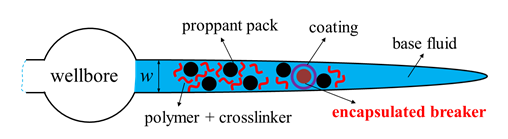
Figure 9: A schematic view of the breaker encapsulation
The time at which breakers take effect are called delay time, after which the \(\textrm{K}\) and \(\textrm{n}\) are both functions of time \(\textrm{t}\) to characterize the time-dependence of \(\mu_a\). For example, Figure 10 indicates that the breaker takes effect after \(120\) seconds of the pumping start.
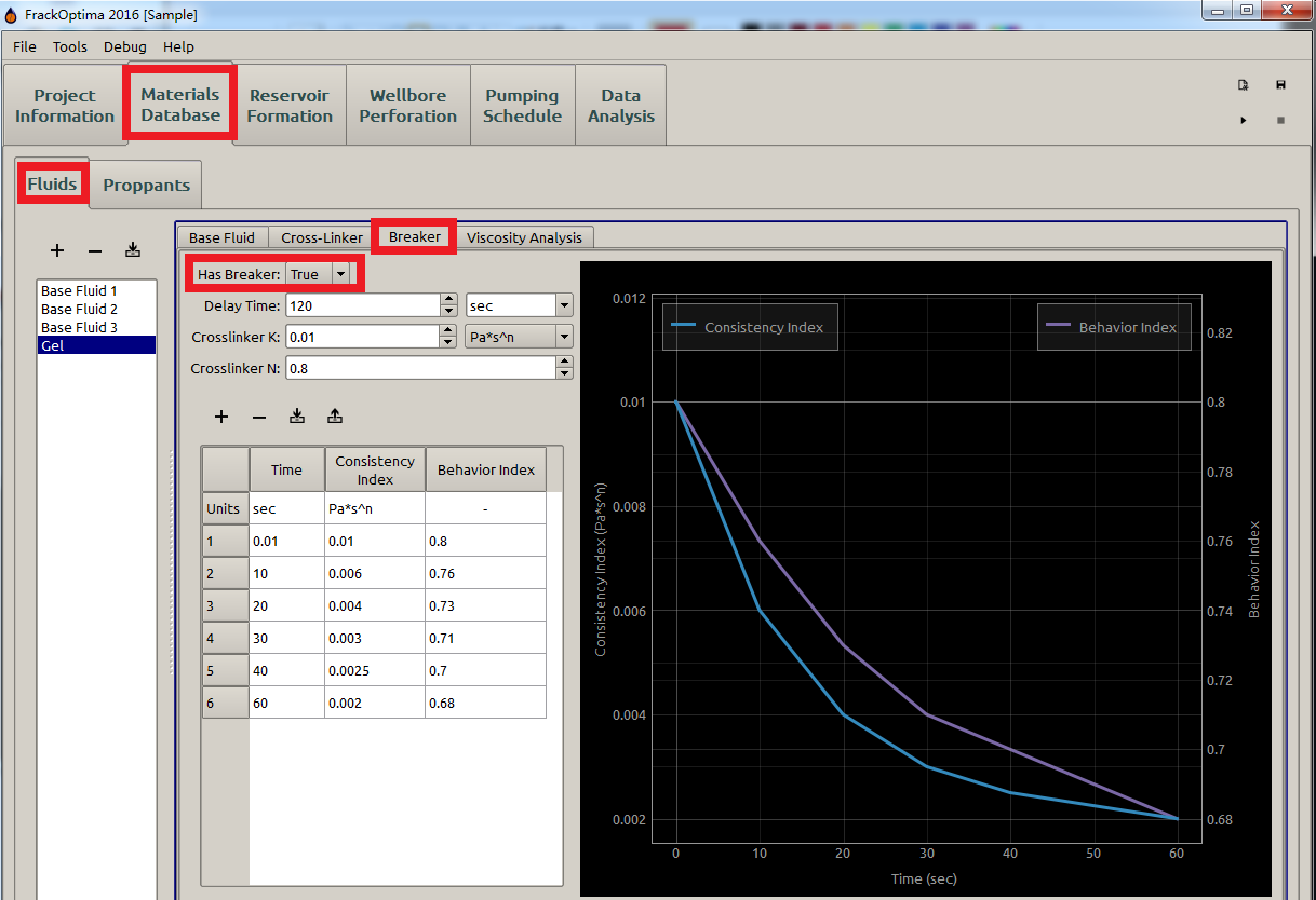
Figure 10: Breaker parameters
\(\textrm{K}\) and \(\textrm{n}\) can be interpreted through experiments .Once a table of the \(\textrm{K}\) and \(\textrm{n}\) at different time is obtained and input, two corresponding curves will be displayed at right.
Note
- The Time in the table and plotting represents the time after the delay time, not the actual time during pumping. For example, \(\textrm{30s}\) means \(\textrm{30s}\) after delay time, which is the \(\textrm{150ths}\) in this case (Delay Time is \(\textrm{120s}\)).
- \(\mathrm{0}\) cannot be an input for Time in the table here since the fracking fluid properties right at the delay time equals to the ones of cross-linker defined in the Cross-Linker subpanel (Figure 8).
- Although the subpanel is named Breaker, the properties listed are the ones of the mixture fracking fluid.
Viscosity Analysis
With parameters defined in Cross-Linker and Breaker, the apparent viscosity of the mixture fracking fluid can be obtained by Eq. (6). With the Input Times defined by the users, the apparent viscosity at different time will be available in Output and displayed as shown in Figure 11.
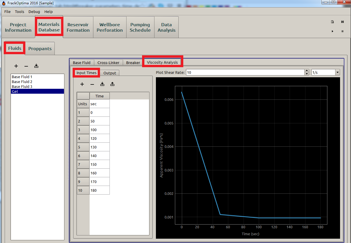
Figure 11: Viscosity analysis
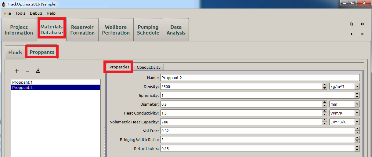
Proppant Properties
Proppants are solid particles contained in fracking fluids that keep hydraulic fractures open during and following a fracturing treatment. Proppants are typically made from treated sand or man-made ceramic materials.
Name
Similar to Name in Fluid subpanels, proppants have names which are used in the Pumping Schedule panel. Proppant names must be unique.
Density
The definition of density can be referred to here.
A typical density for proppants ranges from \(\textrm{1560}\) to \(\textrm{2050 kg}/\textrm{m}^3\) [11] [12].
Sphericity
Sphericity, usually denoted by \(\Psi\), is a measure of how spherical an object is. It is defined by Wadell as the ratio of the surface area of a sphere with the same volume as the given object to the surface area of the object:
where:
- \(\textrm{V}_p\) is the volume of the object
- \(\textrm{A}_p\) is the surface area of the object
The sphericity of a sphere is \(\textrm{1}\) and any object that is not a sphere has sphericity less than \(\textrm{1}\). A typical value of the sphericity for man-made ceramic proppant may be \(\textrm{1}\), i.e. they can be assumed as perfect spheres in the simulation.
Diameter, m
When the sphericity is less than \(\textrm{1}\), the proppant diameter \(\textrm{d}\) is the diameter of a sphere having the same volume as the proppant particle defined by:
where \(\textrm{V}\) denotes the volume.
\(\textrm{0.5} \sim \textrm{2mm}\) is an acceptable proppant diameter value [13].
Both sphericity (shape effect) and the proppant concentration affect the proppant settling velocity along the wellbore and fractures. The Thomas empirical equation may be used to predict the proppant settling velocity without considering the shape effect [14]:
where:
- \(c\) is the volumetric fraction (concentration) of proppant
- \(v_0\) is the settling velocity of a single spherical particle
- \(v_c\) is the settling velocity of spherical particles in a concentration \(c\)
The effect of an irregular shape may be considered by using the correlated equation [15]:
where:
- \(\Psi\) is the sphericity of proppant particle
- \(d\) is the equivalent diameter of proppant particle
- \(\mu_a\) is the apparent viscosity of the fluid
- \(\rho_f\) and \(\rho_p\) is the density of the fluid and proppant, respectively
Eqn (11) and Eqn (12) are coupled to model the proppant settling in FrackOptima.
Heat Conductivity
The definition of heat conductivity can be referred to here .
At room temperature (about \(300 \mathrm{K}\)), the proppant heat conductivity may be approximated as that of saturated sand, which is \(2 \sim 4 \mathrm{W}/(\mathrm{m} \bullet \mathrm{K})\) [3] .
Volumetric Heat Capacity
The definition of volumetric heat capacity can be referred to here .
At room temperature (about \(300 \textrm{K}\)), a value of around \(1.6 \textrm{MJ}/(\textrm{K} \bullet \textrm{m^3})\) is be reasonable for the proppant volumetric heat capacity [16] .
Packed Volume Fraction
The Packed Volume Fraction is a parameter that characterizes the maximum volume fraction of solid objects when they are packed randomly. It is the volume fraction of solid particles when they are closed-packed. A basic packing model is the closed sphere packing model, in which the minimum packed volume fraction is about \(\textrm{0.52}\) for close-packed simple cubic as shown in Figure 12 [17]:
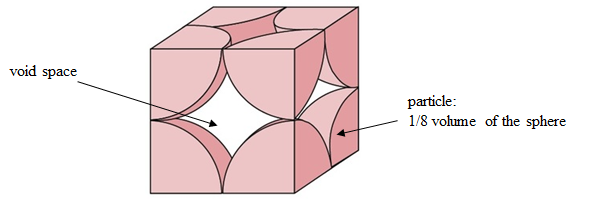
Figure 12: Close-packed simple cubic
The maximum packed volume fraction for a closed sphere packing model is \(\textrm{0.74}\), which is called face-centered cubic or FCC, as shown in Figure 13 [18]. Thus, it is reasonable to input a value between \(\textrm{0.52}\) and \(\textrm{0.74}\) for packed volume fraction. A typical value can be chosen as \(0.635\) [19].
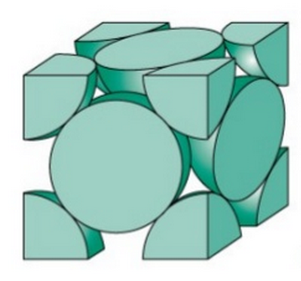
Figure 13: Face-centered cubic
Bridging Width Ratio
Generally, higher proppant concentrations result in greater fracture conductivity, which is beneficial to production. However, there are limits to proppant concentrations that can be placed: if concentrations become too high the proppant will begin to bridge off in the fracture, creating a screen-out which stops propagation of the fracture [20].
It has been found that the ratio of the perforation diameter to average particle diameter is a critical factor to determine the bridging. For example, if the ratio is \(\textrm{1} \sim \textrm{2}\), bridging occurs at a low proppant concentration ranging \(\textrm{0.5} \sim \textrm{1 lbm/gal}\) , while the ratio is greater than \(\textrm{6}\), bridging does not occur even at proppant concentrations of \(\textrm{30 lbm/gal}\) (volume concentration \(\textrm{0.58}\)) [21]. Thus, \(\textrm{6}\) may be an appropriate input for this Bridging Width Ratio.
Retard Index
The proppants travel at a mean velocity \(v_p\) within the fracturing fluid at a mean velocity \(v_f\) (Figure 14).
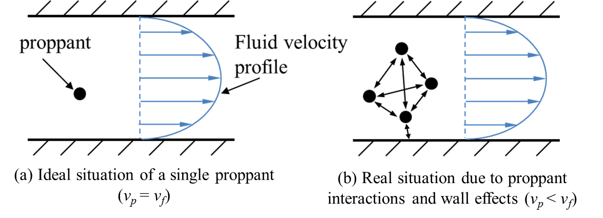
Figure 14: Transportation of proppants
The two velocities are related with the equation:
where, \(v_s\) represents the velocity retardation (difference between \(v_p\) and \(v_f\)).
Ideally, a single proppant travels at the same velocity as the fluid ( (Figure 14 (a)). However, the interactions between proppants and the wall effects slow down the proppants, leading to the velocity retardation \(v_s\). In FrackOptima, a parameter called Retard Index is introduced to represent the \(v_s\), which ranges from \(0\) (\(v_s\) =0) to \(1\) (\(v_p\) = 0).
Proppant Conductivities
| [1] | Laminar Shear,`Wikipedia<http://en.wikipedia.org/wiki/Viscosity#mediaviewer/File:Laminar_shear.svg>`_ Licensed under CC 3.0 |
| [2] | http://en.wikipedia.org/wiki/List_of_thermal_conductivities#cite_note-Marble-Institute-52 |
| [3] | (1, 2) http://www.engineeringtoolbox.com/thermal-conductivity-d_429.html |
| [4] | http://www.engineeringtoolbox.com/water-thermal-properties-d_162.html |
| [5] | Petty, Xu: The effects of proppant concentration on the rheology of slurries for hydraulic fracturing-A review, UCR Undergraduate Research Journal (2010) |
| [6] | Govier, Aziz: The flow of complex mixtures in pipes. Van Nostrand Reinhold company, New York (1972), pp. 98 |
| [7] | Walters, etc.: Kinetic rheology of hydraulic fracturing models, SPE-71660 (2001) |
| [8] | Marquardt, etc.: Delayed breaker systems improve fracture conductivity, PETSOC-91-93 (1991) |
| [9] | (1, 2) King, etc.: Encapsulated breaker for aqueous polymer fluids, PETSOC-90-89 (1990) |
| [10] | Lo, etc.: Encapsulated breaker release rate at hydrostatic pressure at elevated temperatures, SPE-77744 (2002) |
| [11] | “An introduction to proppants and their properties” by Carbo Ceramics |
| [12] | http://pwaa000102.psiweb.com/English/tools/topical_ref/tr_physical.html |
| [13] | Gert Bechmann: Measuring the size and shape of frac sand and other proppants, Webinar presentation of Retsch Technology (2012) |
| [14] | Thomas: Transport characteristics of suspensions: VII. Relations of hindered settling floc characteristics to rheologicial parameters. J. of AIChe, 9(3), 310-316 (1963) |
| [15] | Chien: Settling velocity of irregularly shaped particles, SPE-26121 (1994) |
| [16] | http://www.engineeringtoolbox.com/specific-heat-solids-d_154.html |
| [17] | http://www.chegg.com/homework-help/questions-and-answers/q-hypothetical-metal-simple-cubic-crystal-structure-shown-figure–atomic-weight-745-g-mol–q3488040 |
| [18] | http://en.wikipedia.org/wiki/Atomic_packing_factor |
| [19] | http://en.wikipedia.org/wiki/Atomic_packing_factor |
| [20] | Boyer, Guazzelli and Pouliquen. Unifying suspension and granular rheology. Physical Review Letters. 107 (18) 18-28 (2011) |
| [21] | Gruesbeck, Collins: Particle transport through perforations, SPE-26121-PA (1982) |