Surface Pressure Computation
Introduction
The different pressures during a typical fracturing treatment is illustrated in Figure 1.
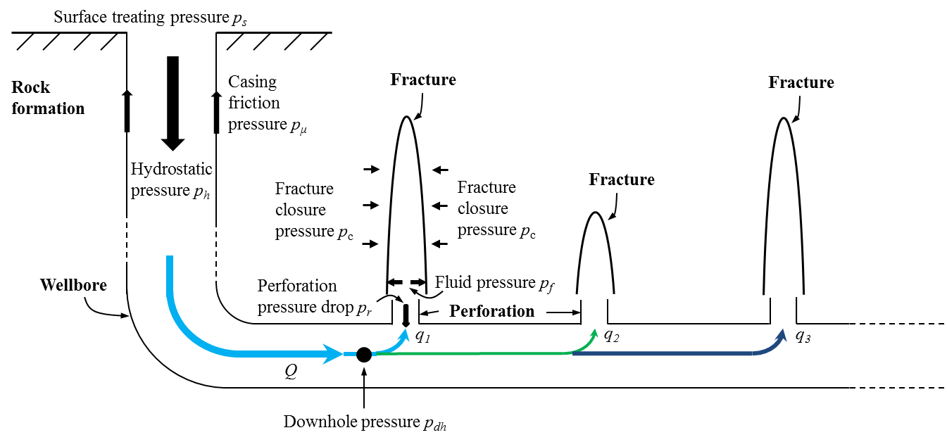
Figure 1: Pressures in a typical fracturing treatment
where:
- \(Q\) is the total volumetric injection rate of the fracturing fluid being pumped into the wellbore;
- \(q\) is the volumetric injection rate of the fracturing fluid being pumped through a specific injection site;
- the subscript \(i\) represents the \(i\) th injection sit.
FrackOptima computes the downhole pressure \(p_{dh}\) during a fracturing treatment. The surface pressure \(p_s\) can be interpreted by:
where, the gravitational static pressure \(p_h\) can be calculated accurately with known fluid and proppant densities.
However, the calculation of the fluid friction pressure \(p_{\mu}\) is not straight forward and requires careful consideration of the effects of various factors on the characterization of fluid friction, the laminar or turbulent flow, the crosslinking process, proppant, and wellbore roughness. And FrackOptima presents the following procedure to model \(p_{\mu}\), leading to obtaining the surface pressure from (1) .
Inputs
The inputs to calculate \(p_{\mu}\) are:
- The pumping schedule, including injection rate, injection volume, etc. See here for a detailed explanation of the pumping schedule.
- The time it takes for a fluid to be crosslinked if the fluid has crosslinker(Figure 2).
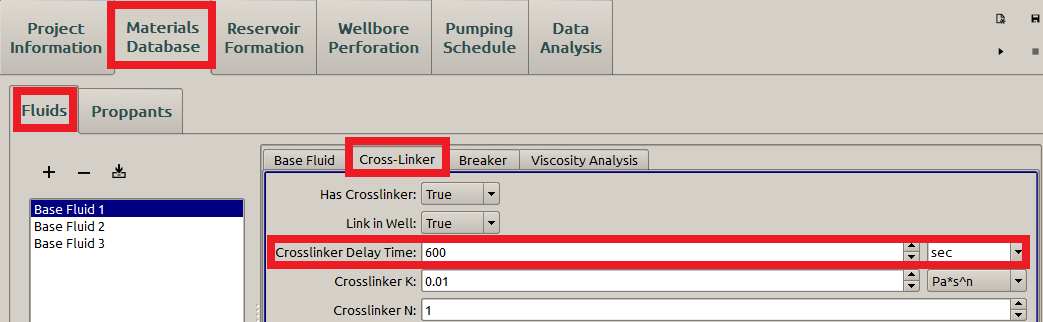
Figure 2: Crosslinker time
Procedure
1. Determine fluid properties
At a given moment, the slurry profile inside the wellbore can be identified according to the pumping schedule. At a particular location, we know the wellbore diameter \(D\) , wellbore roughness \(\epsilon\), slurry density \(\rho\), slurry velocity \(v\), slurry injection time \(t\) (from surface to current location), fluid consistency index \(K\) , fluid behavior index \(n\) , proppant volume fraction \(c\) , and Landel viscosity index \(m\) . Having known these parameters, we need to check whether fluid is crosslinked by comparing fluid injected time \(t\) with the time it takes for a fluid to be crosslinked. Then, we can determine whether the fluid consistency index \(K\) and the behavior index \(n\) are those of the base fluid or the crosslinked one.
2. Compute Reynolds number
The Reynolds number \(Re\) is calculated by:
where, the \(\mu_{eff}\) is the effective viscosity that can be calculated by:
or
Then, we can check if it is laminar or turbulent flow:
if \(Re<2100\) : laminar flow;
if \(Re\ge2100\) : turbulent flow.
3. Determine Fanning friction factor
If the fluid flow is laminar, the Fanning friction factor \(f\) can be obtained:
If the fluid flow is turbulent, \(f\) is solved iteratively from:
For this part, you may check wellbore roughness for details.
4. Compute the friction pressure gradient
The friction pressure gradient (pressure drop per length of the wellbore) is:
The final total friction pressure is then computed by:
where, \(\lambda\) is the friction factor that is used as a correlation factor to better match the surface pressure for practical applications.