Wellbore Perforation
Introduction
This panel specifies the geometry of the wellbore and the injection locations used for hydraulic fracturing. On the left are two input panels, and on the right is a 3D plot of the inputted data.
The two sub-panels, Wells and Injections, contain tables to specify the wellbore geometry and injection locations. Each wellbore is specified by its Well Index. The locations for each wellbore are interpolated and plotted in the 3D plot.
Injections are specified by their location on a well along with their fracturing stage. The Number of Perforations field specifies how many perforations are located at that particular injection point. The Frac Stage field determines in what stage the injection location is active.
Details can be found in the following glossary of parameters.
The parameters in Microseismic subpanel can be found here, and the parameters in Reservoir Stress is explained here.
Wells
Tube Diameter
The Tube Diameter specifies the innermost diameter of the wellbore. In FrackOptima, the thickness of the well does not play a role. A typical value is \(\textrm{50 mm}\).
Wellbore Roughness
When fluid flows through a pipe, it loses energy from friction between the fluid and the pipe wall. In the context of hydraulic fracturing, this friction means extra energy must be expended to pump the fluid. The Fanning friction coefficient \(f\) is a characterization of this friction, and it is defined as:
where:
- \(D\) is the wellbore diameter
- \(\rho\) is the fluid density
- \(v\) is the fluid mean velocity
- \(\triangle p\) is the pressure drop at length \(L\)
For laminar flow, the following equations can be used to predict the Fanning friction coefficient \(f\) and hence the pressure loss:
where:
- \(N'_\mathrm{Re}\) is the Reynold’s number for a power-law fluid
- \(q\) is the flow rate
- \(n\) is the fluid behavior index and \(K\) is the fluid consistency index
For turbulent flow through a rough pipe, the following equation may be used to determine the pressure loss of non-Newtonian fluids [1] :
The relative roughness \(\varepsilon\) is defined from the surface roughness, commonly denoted by \(Ra\), which characterizes the surface texture quantified by the vertical deviations of a real surface from its real form. The relative roughness \(\varepsilon\) is defined by dividing \(Ra\) by the wellbore diameter \(D\):
The wellbore can be assumed perfectly smooth if the wellbore roughness is set to 0.
Min Stress Azimuth
The Min Stress Azimuth is the angle \(\alpha\) between the direction of the minimum horizontal stress \(\sigma_{h,min}\) and the North direction, as shown in Figure 1.
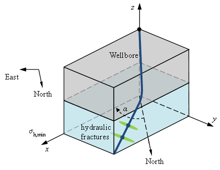
Figure 1: The minimum horizontal stress azimuth
For example, if the min stress direction is North, then the min stress azimuth would be 0 degrees. If the min stress direction is exactly East, then the min stress azimuth would be 90 degrees.
Wellbore Information
The Well Number or Well Index is a name with an integer that defines which well that the table below characterizes. For example, in Figure 2, there are two wells with the Well index Well 1 and Well 2, respectively. Well 1 is the left side well with four injections specified, while Well 2 is the right side vertical one without injections specified. A user can see the corresponding wellbore information in a tabular form when selecting the Well Index. The Well indices are made up of consecutive numbers.

Figure 2: The wellbore information
The brown planes in Figure 2 are the interfaces at Depth \(\textrm{-800 m}\), \(\textrm{0 m}\), \(\textrm{400 m}\), and \(\textrm{800 m}\) defined in Reservoir Formation Interface subpanel.
Injections
Injections are defined as a cluster of perforations on a wellbore. Thus, injection locations are defined for each injection point instead of each perforation. The Injections subpanel is shown as Figure 3.
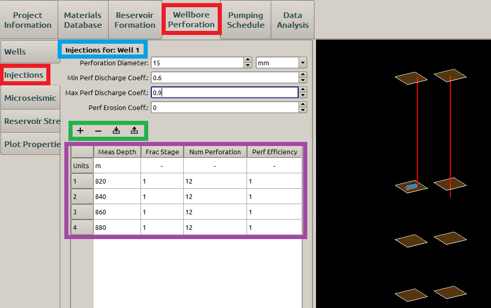
Figure 3: Injection Locations subpanel
Because the Well 1 is selected in the wells subpanel, thus the injection inputs specified here are associated with Well 1 (blue box in Figure 3). Users can also specify injections on other wells by selecting the corresponding ones.
Perforation Diameter
When the fracking fluid flows through the perforation holes the fluid erodes the hole so that the perforation diameter enlarges. The Perforation Diameter input defines the initial diameter of the perforation. A typical value is 10 \(\mathrm{mm}\).
Min and Max Perforation Discharge Coefficient
The discharge coefficient is a dimensionless correction factor for a fluid flow [2] [3] that represents the effect of the perforation entrance shape on the pressure drop [4].
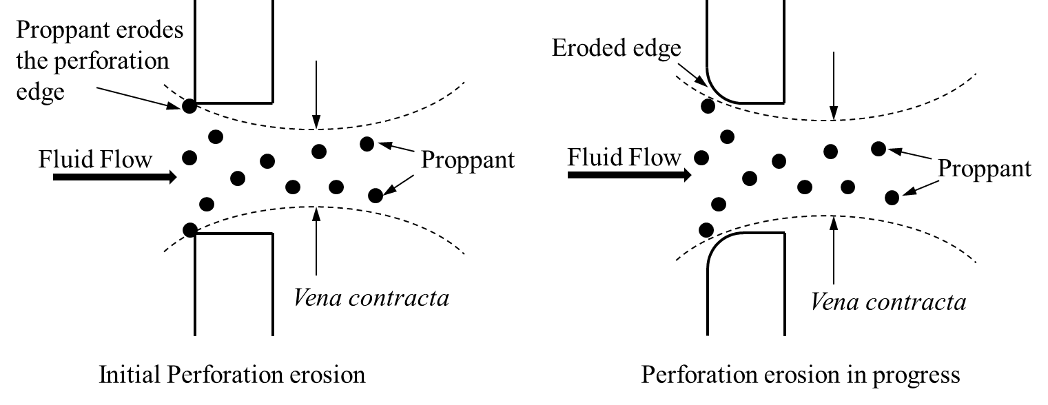
Figure 4: Increasing discharge with perforation erosion [5]
With perforation erosion, the perforation orifice is eroded as shown in Figure 4, resulting in a larger fluid discharge rate and reducing perforation pressure. The Min Perforation Discharge Coefficient represents the initial discharge coefficient of the perforations before erosion and the Max Perforation Discharge Coefficient represent the constant maximum discharge coefficient of a eroded orifice at the later time of the hydraulic fracturing treatment, because Crump’s experiments [5] indicate that the perforation erosion undergoes with a relative constant discharge coefficient at large time. A typical pair of these two parameters is \(0.6\), and \(0.9\).
Perforation Erosion Coefficient
The flow of proppant-laden slurry through a perforation generally results in a change in the geometry through the perforation due to the abrasion process between the proppant and casing. The change in geometry can be significant if a large amount of proppant is pumped with a high injection rate, such as when the limited entry technique is employed in massive hydraulic fracturing along horizontal wells. Accurately predicting fracture geometry requires considering geometric changes in perforations since they cause fluid redistribution among different injection locations. Furthermore, it is also beneficial for an operator to recognize the reduction of pumping pressure due to perforation erosion if such pressure is also used to interpret the possible fracture configuration.
The geometric change of a perforation is assumed to be reflected by the perforation diameter \(D\) and the discharge parameter \(C_d\). Crump’s argument [5] is well accepted [2] \(^-\) [4] that the perforation erosion consists of two mechanisms:
- first, the rounding and smoothing of the entrance to a perforation causes an immediate and significant perforation pressure reduction, when \(C_d\) is dominating the enlargement of both \(D\) and \(C_d\);
- second, the perforation diameter \(D\) increases slowly to cause a further perforation pressure drop at large time with relative constant discharge coefficient (\(C_\mathrm{d,max}\)) .
The rates of change of \(D\) and \(C_d\) are then formulated as:
where:
- \(C\) is the local proppant volume concentration
- \(v\) is the local proppant velocity as the slurry passes through the perforation
- \(\alpha\) and \(\beta\) are two parameters which can be empirically fitted to match the perforation behavior, whose specific values depends on the mechanical properties of the proppant and casing [6].
- \(C_d\) is the discharge coefficient and \(C_\mathrm{d,max}\) is the maximum discharge coefficient
An example of obtaining \(\alpha\) and \(\beta\) for \(\textrm{20/40}\) sand proppant and \(\textrm{N-80}\) casing material combnation (denoted as \(\alpha_0\) and \(\beta_0\)) is available in Ref.6 [6]. And we assume \(\alpha\) and \(\beta\) for other material combinations are proportional to \(\alpha_0\) and \(\beta_0\) with the same constant proportionality \(\lambda\). Then Eqn (5) may be rewritten as:
where:
- \(\lambda\) is the Perforation Erosion Coefficient defined by the user. If it is \(\textrm{0}\), the perforation erosion is excluded during simulation.
- \(\alpha_0\) and \(\beta_0\) are two fixed constants obtained from Ref.6 [6].
Injection Table
The Injection Table (purple box in Figure 3) defines the location of each injection on the wellbore(s) defined in the Wells subpanel.
The Meas Depth represents the measured depth measured from the first depth value of the well (\(\textrm{-800m}\) here in the blue box in Figure 2). This Meas Depth is measured along the wellbore. For example, the \(\textrm{820m}\) in Figure 3 is located \(\textrm{20m}\) from the corner of the horizontal part and the vertical part, because the vertical part is \(\textrm{800m}\).
The Frac Stage determines in what stage the injection location is active. This parameter is going to be used in the pumping-schedule (Fig 5).
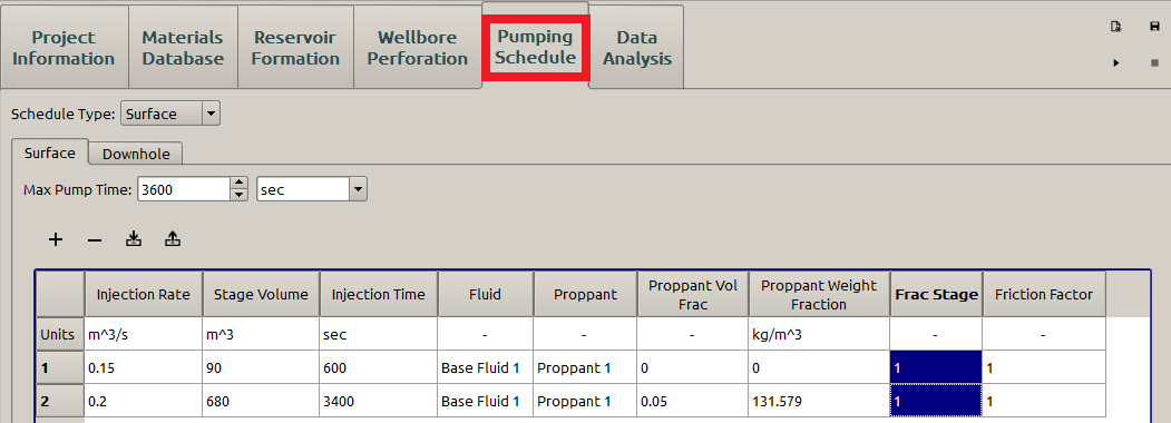
Figure 5: Frac stage in the pumping schedule
The Number of Perforations field specifies how many perforations are located at that particular injection point. When the limited-entry treatment is implemented, it is an significant factor for the treatment.
The Perf Efficiency
Plot Properties
The wellbore plot is a 3D representation of the wellbore and injection location data. The plot controls are located in the Plot Properties subpanel to the left. The six check boxes in that tab specify what is visible on each plot:
Wellbores: Line connecting each given wellbore point
Injections: Spheres representing each injection point
Layers: 3D planes representing the layers specified in the Interface Table
Microseismic: Spheres representing the input from the Microseismic Data subpanel (Fig 6)
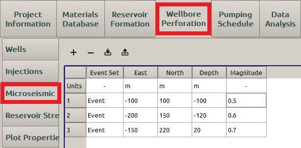
Figure 6: Microseismic data input example
Min Stress Azimuth: the angle between the direction of minimum horizontal stress and the North direction (see here)
Raw Reservoir Stress: representing the input from the Reservoir Stress subpanel
Similar to the Plot Properties subpanel of Reservoir Formation panel, any unchecked items will not displayed at right. Figure 7 is an example with Mini Stress Azimuth and Reservoir Stress unchecked. If the Reservoir Stress is involved, the plotting becomes a little more complicated. Please see here for details.
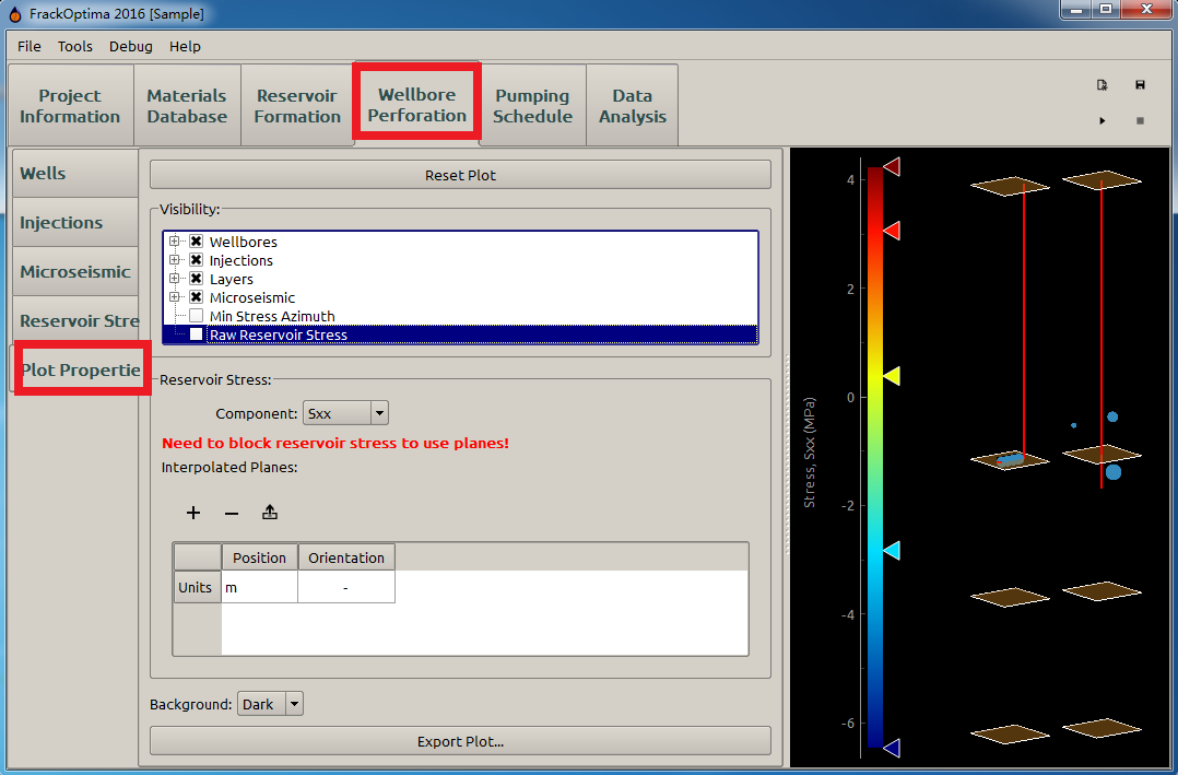
Figure 7: Wellbore and injections plot
The three spheres with different sizes off the wellbores are the plots of the Microseismic data input in Fig 6. Larger size corresponds to larger magnitude.
The Plot Background drop down menu changes the background color of the plot. Finally, the Export button exports the current 3D plot view into an image file.
| [1] | Szilas, Bobok, Navratil: Determination of turbulent pressure loss of Non-Newtonian oil flow in rough pipes, Rheologica Acta, 20, 486-496 (1981) |
| [2] | (1, 2) Lord, Shah, etc. : Study of perforation friction pressure employing a large-scale fracturing flow simulator, SPE-28508 (1994) |
| [3] | El-Rabba, Shah, Lord: New perforation pressure-loss correlations for limited-entry fracturing treatments. SPE-54533 (1999) |
| [4] | (1, 2) Romero, Mack, Elbel: Theoretical model and numerical investigation of near-wellbore effects in hydraulic fracturing. SPE-30506 (1995) |
| [5] | (1, 2, 3) Crump, Conway: Effects of perforation-entry friction on bottomhole treating analysis, SPE-15474 (1988) |
| [6] | (1, 2, 3) Long, Liu, Xu: Modeling of Perforation Erosion for Practical Hydraulic Fracturing Applications, SPE-174959, accepted (2015) |